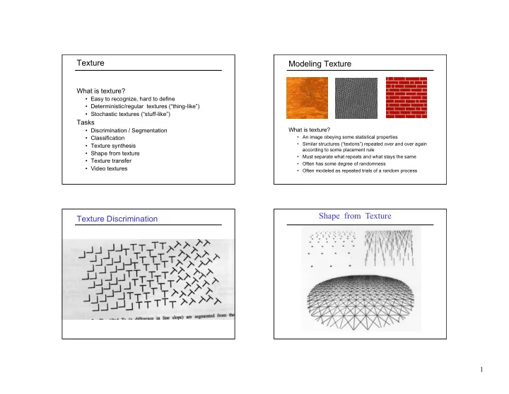
Shape from Texture Texture Discrimination 1 Texture Texture - - PowerPoint PPT Presentation

SLIDE 1

1

Texture

What is texture?

• Easy to recognize, hard to define
• Deterministic/regular textures (“thing-like”)
• Stochastic textures (“stuff-like”)

Tasks

• Discrimination / Segmentation
• Classification
• Texture synthesis
• Shape from texture
• Texture transfer
• Video textures

Modeling Texture

What is texture?

• An image obeying some statistical properties
• Similar structures (“textons”) repeated over and over again

according to some placement rule

• Must separate what repeats and what stays the same
• Often has some degree of randomness
• Often modeled as repeated trials of a random process

Texture Discrimination

Shape from Texture

SLIDE 2

2

Texture

• Texture is often “stuff” (as opposed to “things”)
• Characterized by spatially repeating patterns
• Texture lacks the full range of complexity of

photographic imagery, but makes a good starting point for study of image-based techniques

radishes rocks yogurt

Texture Synthesis

• Goal of texture synthesis: Create new samples of a

given texture

• Many applications: virtual environments, hole-

filling, inpainting, texturing surfaces, image compression

The Challenge

• Need to model the whole

spectrum, from regular to stochastic textures

regular stochastic Both?

Method 1: Copy Blocks of Pixels

Photo Pattern Repeated

Visual artifacts at block boundaries

SLIDE 3

3

Statistical Modeling of Texture

• Assume stochastic model of texture (Markov

Random Field)

• Assume Stationarity: the stochastic model is the

same regardless of position in the image

stationary texture non-stationary texture

Markov Chain

• Markov Chain

– a sequence of random variables x1 , x2 , …, xn – xt is the state of the model at time t – Markov assumption: each state is dependent only on the previous one

• dependency given by a conditional probability:

– The above is actually a first-order Markov chain – An Nth-order Markov chain:

x2 x1 x3 x5 x4 P(xt | xt-1 ) P(xt | xt-1, …, xt-n )

Markov Random Field

A Markov Random Field (MRF)

• Generalization of Markov chains to two or more dimensions

First-order MRF:

• Probability that pixel X takes a certain value given the values
• f neighbors A, B, C, and D:

D C X A B X * * * * * * * * X * * * * * * * * * * * *

• Higher-order MRFs have larger neighborhoods, e.g.:

P(X | A, B, C, D)

Statistical Modeling of Texture

• Assume stochastic model of texture (Markov

Random Field)

• Assume Stationarity: the stochastic model is the

same regardless of position

• Assume Markov (i.e., local) property :

p(pixel | rest of image) = p(pixel | neighborhood)

?

SLIDE 4

4

Motivation from Language

• Shannon (1948) proposed a way to generate

English-looking text using N-grams:

– Assume a Markov model – Use a large text corpus to compute probability distributions of each letter given N–1 previous letters – Starting from a seed, repeatedly sample the conditional probabilities to generate new letters – Can use whole words instead of letters too

Mark V. Shaney (Bell Labs)

• Results (using alt.singles corpus):

– “As I've commented before, really relating to someone involves standing next to impossible.” – “One morning I shot an elephant in my arms and kissed him.” – “I spent an interesting evening recently with a grain of salt.”

• Notice how well local structure is preserved!

– Now let’s try this in 2D using pixels

Efros & Leung Algorithm

Idea initially proposed in 1981 (Garber ’81), but dismissed as too computationally expensive

• A. Efros and T. Leung, Texture synthesis by non-parametric

sampling, Proc. ICCV, 1999

Synthesizing One Pixel

– What is P(x | neighborhood of pixels around x) ? – Find all the windows in the image that match the neighborhood

• consider only pixels in the neighborhood that are already

filled in – To synthesize pixel x, pick one matching window at random and assign x to be the center pixel of that window sample image Generated image

SAMPLE x

SLIDE 5

5

Efros & Leung Algorithm

• Assume Markov property, sample from P(x | Nbr(x))

– Building explicit probability tables is infeasible x

Synthesizing a pixel

non-parametric sampling

Input image

– Instead, we search the input image for all sufficiently similar neighborhoods and pick one match at random

Really Synthesizing One Pixel

sample image

– An exact neighborhood match might not be present – So we find the best matches using “SSD error” and randomly choose between them, preferring better matches with higher probability SAMPLE

Generated image

x

Computing P(x | Nbr(x))

• Given output image patch w(x) centered

around pixel x

• Find best matching patch in sample image:
• Note: normalize d by number of known pixels in w(x)
• Find all image patches in sample image that

are close matches to best patch:

• Compute a histogram of all center pixels in Ω
• Histogram = conditional pdf of x

sample w best

I w x w d w ⊂ = ) ), ( ( min arg ) ), ( ( ) 1 ( ) ), ( ( | { ) (

best

w x w d w x w d w x ε + < = Ω

sum( sum( .− ).^2))

Finding Matches

• Sum of squared differences (SSD)
• r, in Matlab:

|| − ||2

SLIDE 6

6

|| .*( .– )||

2

Finding Matches

• Sum of squared differences (SSD)

– Gaussian-weighted to make sure closer neighbors are in better agreement

• The picture shows a smoothing

kernel proportional to (which is a reasonable model of a circularly symmetric fuzzy blob)

Slide by D.A. Forsyth

Gaussian Filtering

2 2 2

2σ y x

e

+ −

Growing Texture

– Starting from the initial configuration, “grow” the texture

• ne pixel at a time

– The size of the neighborhood window is a parameter that specifies how stochastic the user believes the texture to be – To grow from scratch, we use a random 3 x 3 patch from input image as seed

Details

• Random sampling from the set of candidates
• vs. picking the best candidate
• Initialization for blank output image

– Start with a “seed” in the middle and grow outward in layers

• Hole filling: Growing in “onion skin” order

– Within each “layer”, pixels with the largest number of known-neighbors are synthesized first – Normalize error by the number of known pixels – If no close match can be found, the pixel is not synthesized until the end

SLIDE 7

7

Varying Window Size

input

Varying Window Size

Increasing window size

Synthesis Results

french canvas raffia weave

Results

aluminum wire reptile skin

SLIDE 8

8

Results

white bread brick wall

Results

wood granite

Hole Filling Extrapolation

SLIDE 9

9

Failure Cases

Growing “garbage” Verbatim copying

Homage to Shannon

Summary of Efros and Leung Algorithm

• Advantages:

– conceptually simple – models a wide range of real-world textures – naturally does hole-filling

• Disadvantages:

– it’s greedy – it’s slow – it’s heuristic

Accelerating Texture Synthesis

• For textures with large-scale

structure, use a Gaussian pyramid to reduce required neighborhood size

L.-Y. Wei and M. Levoy, "Fast Texture Synthesis using Tree-structured Vector Quantization," SIGGRAPH 2000

SLIDE 10

10

Another Property of Gaussians

• Cascading Gaussians: Convolution of a

Gaussian with itself is another Gaussian

– So, we can first smooth an image with a small Gaussian – Then, we convolve that smoothed image with another small Gaussian and the result is equivalent to smoothing the original image with a larger Gaussian – If we smooth an image with a Gaussian having standard deviation σ twice, then we get the same result as smoothing the image with a Gaussian having standard deviation √2σ

2σ

Pyramids

• Useful for representing images at multiple

“scales”

• Pyramid is built using multiple copies of

image

• Each level in the pyramid is an image with

1/4 the number of pixels of previous level, i.e., each dimension is 1/2 resolution of previous level

Pyramids

SLIDE 11

11

Reduce Gaussian Pyramids

) 2 , 2 ( ) , ( ) , (

2 2 2 2 1

n v m u g n m w v u g

m n l l

+ + = ∑ ∑

− = − = −

] [

1 −

=

l l

g REDUCE g

Expand Gaussian Pyramids

] [

1 , , −

=

n l n l

g EXPAND g

) 2 , 2 ( ) , ( ) , (

2 2 2 2 1 , ,

q v p u g q p w v u g

p q n l n l

− − = ∑ ∑

− = − = −

SLIDE 12

12

Convolution Mask

Commonly used masks: [.05, .25, .4, .25, .4]

• r 1/20 [1, 5, 8, 5, 1]
• r 1/16 [1, 4, 6, 4, 1]

)] 2 ( ), 1 ( ), ( ), 1 ( ), 2 ( [ w w w w w − −

Exploit separability property of Gaussian filtering

Accelerating Texture Synthesis

• For textures with large-scale

structure, use a Gaussian pyramid to reduce required neighborhood size

– Low-resolution image is synthesized first – For synthesis at a given pyramid level, the neighborhood consists of already generated pixels at this level plus all neighboring pixels at the lower-resolution level

L.-Y. Wei and M. Levoy, "Fast Texture Synthesis using Tree-structured Vector Quantization," SIGGRAPH 2000

Gaussian Pyramid

High resolution Low resolution p

Image Quilting

• Observation: neighbor pixels are highly correlated

Input image

non-parametric sampling

B Idea: unit of synthesis = block of pixels

• Exactly the same as Efros & Leung but now we want

P(B|Nbr(B)) where B is a block of pixels

• Much faster: synthesize all pixels in a block at once

Synthesizing a block

• A. Efros and W. Freeman, Image quilting for texture synthesis and transfer,
• Proc. SIGGRAPH, 2001

SLIDE 13

13

Input texture

B1 B2

Random placement

• f blocks

block

B1 B2

Neighboring blocks constrained by overlap

B1 B2

Minimum error boundary cut

Main Idea

• The “Plagiarist’s Algorithm”

– Copy as much of the source image as you can – Then try to cover up the evidence

• Rationale:

– Texture blocks are by definition correct samples

• f texture so the only problem is connecting them

together

Algorithm

– User picks size of block and size of overlap – Synthesize blocks in raster order – Search input texture for all blocks that satisfy overlap constraints (above and left)

• Overlap error SSD < threshhold

– Paste new block into resulting texture

• Use Dynamic Programming to compute minimum error

boundary cut

• min. error boundary

Minimum Error Boundary

• verlapping blocks

vertical boundary

_

=

2

• verlap error

SLIDE 14

14

Dynamic Programming

• Linear time algorithm for solving sequential decision

(optimal path) problems

1 2 3 1 2 3 1 2 3

1 = t 2 = t 3 = t 1 = i 2 = i 3 = i

1 2 3 T t =

…

How many paths through this trellis?

T

3

Assume cost can be decomposed into stages

Dynamic Programming

1 2 3 1 2 3 1 2 3

1 − t

C

t

C

1 + t

C

12

Π

22

Π

32

Π States:

1 = i 2 = i 3 = i

Dynamic Programming

1 2 3 1 2 3 1 2 3

Principle of Optimality for an n-stage assignment problem:

)) ( ( min ) (

1 i

C j C

t ij i t −

+ Π =

2 = j 1 = i 2 = i

3 = i

1 − t

C

t

C

1 + t

C

12

Π

22

Π

32

Π

22

Π

32

Π 2 ) 2 ( =

t

b

Dynamic Programming

1 2 3 1 2 3 1 2 3

)) ( ( min arg ) ( )) ( ( min ) (

1 1

i C j b i C j C

t ij i t t ij i t − −

+ Π = + Π =

remember best predecessor

2 = j 1 = i 2 = i

3 = i

1 − t

C

t

C

1 + t

C

SLIDE 15

15

Minimum Error Boundary

_

=

2

• verlap error
• Let i = 1, …, number of columns of overlap
• Let t = 1, …, number of rows in overlap

SLIDE 16

16

Failures

SLIDE 17

17

input image

Wei & Levoy Efros & Freeman Wei & Levoy Efros & Freeman

input image

Wei & Levoy Efros & Freeman

input image

Political Texture Synthesis!

SLIDE 18

18

Texture Transfer

• Take the texture from one source “palette”

image and “paint” it onto another “target” image – This requires separating texture and shape – That’s HARD, but we can cheat

• Just add another constraint when picking a

block: similarity to target image at that position

• Error = α(overlap error w/ palette block) +

(1-α)(diff w/ target image)

• Here, diff w/ target image = SSD between

palette texture block and intensity in block

• f target face image
• Iterate using successively smaller block sizes

Here, bright patches of rice should match bright patches of face, and dark patches match too

+ = + =

parmesan rice

+ =

Target image Source palette image Output image Here, diff w/ target image = SSD between blurred palette texture block and blurred intensity in block of target face image

SLIDE 19

19

+ =

Source palette Target

= +

Target Palette

Efros and Freeman Alg. Summary

• Quilt together patches of input image

– randomly (texture synthesis) – constrained (texture transfer)

• Image Quilting

– No filters, no multi-scale, no one-pixel-at-a-time! – fast and very simple – Results are not bad

Extension: Texture Transfer Using Objects as Primitives

Lorenzo De Carli, UW

• Throughout the centuries, many artists created

stunning visual effects by rendering well-known physical objects using combinations of other

• bjects.
• The first to do so was probably the 16th century

Italian painter Giuseppe Arcimboldo

• The technique is also popular among modern

artists such as Octavio Ocampo

SLIDE 20

20

Giuseppe Arcimboldo Method

• Small images of a user-specified library of objects

are used as "macropixels" to render the image

• The algorithm works by computing all possible

matchings of the objects in the library with the source image – computing the pixel-by-pixel difference (SSD) between the colors of the two images

• The closest matchings are chosen and used to

generate the result image

Library of Object Images

Matching an Object with an Image Patch

SLIDE 21

21

Full Image Rendering Multiple Region Rendering Results Extension: Texture Synthesis from Non-Fronto-Parallel Textures

Input Output Saurabh Goyal, UW-Madison

SLIDE 22

22

Extension: Texture Synthesis on Surfaces

L.-Y. Wei and M. Levoy, “Texture Synthesis over Arbitrary Manifold Surfaces,” SIGGRAPH 2001

+

Input Texture Input Mesh Result

Extension: 3D Texture Synthesis

• J. Kopf et al., “Solid Texture Synthesis from 2D Exemplars,” SIGGRAPH 2007

Multiscale Texture Synthesis

Input: Multiscale texture graph Output: Multiscale texture image

• C. Han et al., SIGGRAPH 2008

A Simple Graph

SLIDE 23

23

Image Analogies

Hertzmann et al., SIGGRAPH 2001

Input image A Input image A´ Input image B Output image B´

Image Analogies

Unfiltered source Filtered source Unfiltered target Filtered target

Image Analogies: Assumptions

• Image A´ is assumed to have been created

from A by applying some unknown filter

• Images A and A´ are assumed to be

registered, i.e., the colors around pixel p in A correspond to the colors around pixel p in A´, though transformed via some image filter

• Each pixel has an associated feature vector

specifying color, luminance, and various filter outputs

• Implemented as “resynthesizer” in GIMP

The Approach

Unfiltered target Filtered target Unfiltered source Filtered source

SLIDE 24

24

The Approach

Unfiltered source Filtered source Unfiltered target Filtered target

How to Select Best Pixel for B´(q)?

• Nearest-Neighbor Match: Given F(q) =

concatenation of feature vectors around q in B and B´ at levels l and l-1, find pixel p in A such that F(p) is closest match to F(q) (using Gaussian weighted SSD)

• Coherence Match: Find pixel r in A such

that F(r) is closest match to F(q) for all r’s used to synthesize already synthesized pixels in neighborhood of q

• Pick “best” of p and r

Results: Blur Filter Learning

F(p) = luminance at pixel p in A and A´ in 5 × 5 neighborhood at current level, and 3 × 3 neighborhood at next coarser level

Results: Edge Filter

F(p) = luminance at pixel p

SLIDE 25

25

Texture Synthesis

Source images (A, B) are blank/constant

Unfiltered source Filtered source Unfiltered target Filtered target

Texture Synthesis Texture Transfer

• A and A´ is the same (or A is a blurred version of A´)
• Optional: Use a weight to control the tradeoff between

matching (A, B) and (A´, B´)

Unfiltered source Filtered source Unfiltered target Filtered target

Texture Transfer

Images A and A´ Image B

SLIDE 26

26

Texture Transfer

2 result images, B´ A A´ B B´

Artistic Filters Artistic Filters

A A´ B B´

Artistic Filters

SLIDE 27

27

Artistic Filters

A A´ B B´

Artistic Filters Artistic Filters

A A´ B B´

Artistic Filters

SLIDE 28

28

Artistic Filters

A A´ B B´

Artistic Filters Super-Resolution

A A´ B B´

Super-Resolution

B B´

SLIDE 29

29

Colorization