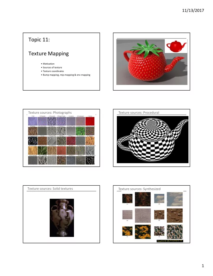
Topic 11: Texture Mapping Motivation Sources of texture - PDF document

11/13/2017 Topic 11: Texture Mapping • Motivation • Sources of texture • Texture coordinates • Bump mapping, mip‐mapping & env mapping Texture sources: Photographs Texture sources: Procedural Texture sources: Solid textures Texture sources: Synthesized 1

11/13/2017 Texture coordinates Original Synthesized How does one establish correspondence? (UV mapping) Original Synthesized Aliasing During Texture Mapping MIP‐Mapping: Basic Idea aliasing Given a polygon, use the texture image, where the projected polygon best matches the size of the polygon on screen. Bump mapping Environment Map Render a 3D scene as viewed from a central viewpoint in all directions (as projected onto a sphere or cube). Then use this rendered image as an environment texture… an approximation to the appearance of highly reflective objects. 2

11/13/2017 Environment Mapping Cube Environment Mapping Local vs. Global Illumination All surfaces are not created equal Specular surfaces Local Illumination Models • e.g. mirrors, glass balls e.g. Phong • An idealized model provides ‘perfect’ reflection • Model source from a light reflected once off a surface Incident ray is reflected back as a ray in a single towards the eye direction • Indirect light is included with an ad hoc “ambient” term Diffuse surfaces which is normally constant across the scene • e.g. flat paint, chalk • Lambertian surfaces Global Illumination Models • Incident light is scattered equally in all directions e.g. ray tracing or radiosity (both are incomplete) • Try to measure light propagation in the scene General reflectance model: BRDF • Model interaction between objects and other objects, objects and their environment Categories of light transport Ray Tracing Specular‐Specular Specular‐Diffuse Traces path of specularly reflected or transmitted Diffuse‐Diffuse (refracted) rays through environment Diffuse‐Specular Rays are infinitely thin Don’t disperse Signature: shiny objects exhibiting sharp, multiple reflections Transport E ‐ S – S – S – D – L. 3

11/13/2017 Ray Tracing Topic 12: Unifies in one framework • Hidden surface removal • Shadow computation Basic Ray Tracing • Reflection of light • Refraction of light • Global specular interaction • Introduction to ray tracing • Computing normals • Evaluating shading model • Computing rays • Spawning rays • Computing intersections • Incorporating transmission • refraction • ray‐triangle • ray‐spawning & refraction • ray‐polygon • ray‐quadric Rasterization vs. Ray Tracing Ray Tracing: Basic Idea Rasterization: ‐project geometry onto image. ‐pixel color computed by local illumination (direct lighting). Ray‐Tracing: ‐project image pixels (backwards) onto scene. ‐pixel color determined based on direct light as well indirectly by recursively following promising lights path of the ray. Ray Tracing: Advantages Ray Tracing: Basic Algorithm For each pixel q • Customizable: modular approach for ray sampling, ray object { Intersections and reflectance models. compute r , the ray from the eye through q ; find first intersection of r with the scene, a point p ; • Variety of visual effects: shadows, reflections, refractions, estimate light reaching p ; indirect illumination, depth of field etc. estimate light transmitted from p to q along r ; } • Parallelizable: each ray path is independent. • Speed vs. Accuracy trade‐off: # and recursive depth of rays cast. 4

11/13/2017 Ray Tracing Imagery Ray Tracing vs. Radiosity Ray tracing setup Topic 12: Basic Ray Tracing • Computing normals • Introduction to ray tracing • Evaluating shading model • Computing rays • Spawning rays • Computing intersections • Incorporating transmission • refraction • ray‐triangle • ray‐spawning & refraction • ray‐polygon • ray‐quadric Computing the Ray Through a Pixel: Steps Ray does not intersect objects e Pixel q in local camera coords [x,y,d,1] T (x,y) Let C be camera to world transform Sanity check e= C [0,0,0,1] T pixel q at (x,y ) on screen is thus C [x,y,d,1] T Ray r has origin at q and direction (q‐e)/|q‐e| . 5

11/13/2017 Ray hits object Shadow test Point in shadow Computing Ray‐Triangle Intersections Topic 12: Let ray be defined parameterically as q + r t for t>=0. Basic Ray Tracing Compute plane of triangle <p1,p2,p3> as a point p1 and normal n= (p2‐p1)x(p3‐p2) . Now (p‐p1).n=0 is equation of plane. Compute the ray‐plane intersection value t by solving • Computing normals • Introduction to ray tracing (q+rt‐p1).n=0 => t= (p1‐q).n /(r.n) • Evaluating shading model • Computing rays • Spawning rays • Computing intersections Check if intersection point at the t above falls within triangle. • Incorporating transmission • refraction • ray‐triangle • ray‐spawning & refraction • ray‐polygon • ray‐quadric • the scene signature 6

11/13/2017 Computing Ray‐Quadric Intersections Computing Ray‐Sphere Intersections ( c ‐ q ) 2 –(( c ‐ q ). r ) 2 =d 2 ‐ k 2 k Solve for k, if it exists. r d c q Intersections: q + r (( c ‐ q ). r +/‐ k) Implicit equation for quadrics is p T Qp =0 where Q is a 4x4 matrix of coefficients. Substituting the ray equation q+r t for p gives us a quadratic equation in t, whose roots are the intersection points. Intersecting Rays & Composite Objects Ray Intersection: Efficiency Considerations • Intersect ray with component objects Speed‐up the intersection process. • • Process the intersections ordered by depth Ignore object that clearly don’t intersect. • to return intersection pairs with the object. Use proxy geometry. • Subdivide and structure space hierarchically. • Project volume onto image to ignore entire Sets of rays. Computing the Normal at a Hit Point Topic 12: • Polygon Mesh: interpolate normals like with Phong Shading. Basic Ray Tracing • Implicit surface f(p)=0 : normal is gradient(f)(p). • Explicit parametric surface f(a,b) : δf(s,b)/ δs X δf(a,t)/ δt • Computing normals • Introduction to ray tracing • Evaluating shading model • Computing rays • Affinely transformed shape: • Spawning rays • Computing intersections • Incorporating transmission • refraction • ray‐triangle • ray‐spawning & refraction • ray‐polygon • ray‐quadric • the scene signature 7

11/13/2017 Evaluating the Shading Model Topic 12: I(q) = L(n,v,l) + G(p)k s Basic Ray Tracing Intensity at q = phong local illum. + global specular illum. • Introduction to ray tracing • Computing normals l q • Evaluating shading model • Computing rays v n G • Spawning rays • Computing intersections • Incorporating transmission • refraction • ray‐triangle • ray‐spawning & refraction • ray‐polygon • ray‐quadric • the scene signature Reflected ray has hit object Reflected ray is sent out from intersection point No reflection Transmitted ray generated for transparent objects 8

11/13/2017 Single reflection Double reflection Ray Tracing with Refraction Topic 12: For transparent objects spawn an additional ray along the refracted direction and recursively return the light Basic Ray Tracing contributed due to refraction. • Computing normals • Introduction to ray tracing • Evaluating shading model • Computing rays • Spawning rays • Computing intersections • Incorporating transmission • refraction • ray‐triangle • ray‐spawning & refraction • ray‐polygon • ray‐quadric • the scene signature Ray Tracing Deficiencies local illumination reflection refraction • Ignores light transport mechanisms involving diffuse surfaces. • Intersection computation time can be long and recursive algorithm can lead to exponential complexity. 9

11/13/2017 Ray Tracing Efficiency Improvements Ray Tracing Improvements: Caustics Bounding volumes Spatial subdivision • Octrees • BSP Ray Tracing Improvements: Image Quality Ray Tracing Improvements: Image Quality Backwards ray tracing Cone tracing • Trace from the light to the surfaces and then from the eye to the surfaces • Models some dispersion effects • “shower” scene with light and then collect it Distributed Ray Tracing • “Where does light go?” vs “Where does light come • Super sample each ray from?” • Blurred reflections, refractions • Good for caustics • Soft shadows • Transport E – S – S – S ‐ D – S – S – S ‐ L • Depth of field • Motion blur Stochastic Ray Tracing Antialiasing – Supersampling How many rays do you need? jaggies w/ antialiasing 1 ray/light 10 ray/light 20 ray/light 50 ray/light point light area light Images taken from http://web.cs.wpi.edu/~matt/courses/cs563/talks/dist_ray/dist.html 10

11/13/2017 Radiosity • Diffuse interaction within a closed environment • Theoretically sound • View independent • No specular interactions • Color bleeding visual effects • Transport E – D – D – D ‐ L 11