Static Electric Fields Static electric fields E ( x, y, z ) vary from - PowerPoint PPT Presentation

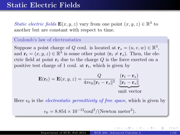
Static Electric Fields Static electric fields E ( x, y, z ) vary from one point ( x, y, z ) ∈ R 3 to another but are constant with respect to time. Coulomb’s law of electrostatics Suppose a point charge of Q coul. is located at r s = ( u, v, w ) ∈ R 3 , and r t = ( x, y, z ) ∈ R 3 is some other point ( r t � = r s ). Then, the ele- ctric field at point r t due to the charge Q is the force exerted on a positive test charge of 1 coul. at r t , which is given by Q ( r t − r s ) E ( r t ) = E ( x, y, z ) = 4 πǫ 0 � r t − r s � 2 � r t − r s � � �� � unit vector Here ǫ 0 is the electrostatic permittivity of free space , which is given by ǫ 0 = 8 . 854 × 10 − 12 coul 2 / (Newton meter 2 ) . Department of ECE, Fall 2014 ECE 206: Advanced Calculus 2 1/22

Static Electric Fields (cont.) Point charges are “singularities” and constitute rather unnatural objects in the theory of electromagnetism. It is much more usual to deal with charge that is diffusely spread through space and described by a charge density scalar field ρ . If ( u, v, w ) is a point within an infinitesimal cube dV ⊂ R 3 , then the total charge enclosed in the cube is given by dQ = ρ ( u, v, w ) dudvdw Thus, the total charge Q , diffusely spread throughout space ac- cording to the density ρ , is � � Q = R 3 dQ = R 3 ρ ( u, v, w ) dudvdw Department of ECE, Fall 2014 ECE 206: Advanced Calculus 2 2/22

Coloumb’s law for diffused charges As a result of the charge dQ the electric field at (x,y,z) is the in- finitesimal vector given by 1 ( x − u ) i + ( y − v ) j + ( z − w ) k d E ( x, y, z ) = [( x − u ) 2 + ( y − v ) 2 + ( z − w ) 2 ] 3 / 2 ρ ( u, v, w ) dudvdw, 4 πǫ 0 with ( u, v, w ) being any point in dV . Our goal is to determine the total electric field at ( x, y, z ) as a result of all the charge contained within R 3 . Specifically, � E ( x, y, z ) = R 3 d E ( x, y, z ) = � � 1 � ( x − u ) ρ ( u, v, w ) [( x − u ) 2 + ( y − v ) 2 + ( z − w ) 2 ] 3 / 2 dudvdw i + 4 πǫ 0 R 3 � � 1 � ( x − v ) ρ ( u, v, w ) + j + [( x − u ) 2 + ( y − v ) 2 + ( z − w ) 2 ] 3 / 2 dudvdw 4 πǫ 0 R 3 � � 1 � ( x − w ) ρ ( u, v, w ) + [( x − u ) 2 + ( y − v ) 2 + ( z − w ) 2 ] 3 / 2 dudvdw k . 4 πǫ 0 R 3 Department of ECE, Fall 2014 ECE 206: Advanced Calculus 2 3/22

Coloumb’s law for diffused charges (cont.) Let us define � 1 ρ ( u, v, w ) Ψ( x, y, z ) := − [( x − u ) 2 + ( y − v ) 2 + ( z − w ) 2 ] 1 / 2 dudvdw 4 πǫ 0 R 3 Observe � � ρ ( u, v, w ) ( x − u ) ρ ( u, v, w ) ∂ = − [( x − u ) 2 + ( y − v ) 2 + ( z − w ) 2 ] 3 / 2 , [( x − u ) 2 + ( y − v ) 2 + ( z − w ) 2 ] 1 / 2 ∂x � � ρ ( u, v, w ) ( y − v ) ρ ( u, v, w ) ∂ = − [( x − u ) 2 + ( y − v ) 2 + ( z − w ) 2 ] 3 / 2 , [( x − u ) 2 + ( y − v ) 2 + ( z − w ) 2 ] 1 / 2 ∂y � � ∂ ρ ( u, v, w ) ( z − w ) ρ ( u, v, w ) = − [( x − u ) 2 + ( y − v ) 2 + ( z − w ) 2 ] 3 / 2 , [( x − u ) 2 + ( y − v ) 2 + ( z − w ) 2 ] 1 / 2 ∂z for all ( x, y, z ). Department of ECE, Fall 2014 ECE 206: Advanced Calculus 2 4/22

Coloumb’s law for diffused charges (cont.) Recalling the gradient operator, we then have ∇ Ψ( x, y, z ) = ∂ Ψ ∂x ( x, y, z ) i + ∂ Ψ ∂y ( x, y, z ) j + ∂ Ψ ∂z ( x, y, z ) k . Then, it is straightforward to see that ∀ ( x, y, z ) ∈ R 3 . E ( x, y, z ) = ∇ Ψ( x, y, z ) , Thus, an electric field arising from charge diffusely distributed through space according to a specified charge density field ρ is conservative. It immediately follows that the above electric field is irrotational, viz. ∇ × E = 0 . Department of ECE, Fall 2014 ECE 206: Advanced Calculus 2 5/22

Gauss’ law for static electric fields Gauss’ law for static electric fields Suppose that E is the electric field arising from the charge density ρ . Then, for any region Ω ⊂ R 3 with the closed outwardly oriented sur- face S as boundary, we have � � E · d A = 1 ρ dV. ǫ 0 S Ω According to Gauss’ law the total flux of E through S does not depend on the “outside” charge and is determined exclusively by the charge inside Ω. Gauss’ law is really just Coulomb’s law but stated in more esote- ric mathematical language. Department of ECE, Fall 2014 ECE 206: Advanced Calculus 2 6/22

Differential form of Gauss’ law Gauss’ law is a global statement since it gives an aggregate or net property of the electric field E . Let’s use the divergence theorem to rewrite Gauss’ law in a local or differential form which says something about E ( x, y, z ) at eve- ry individual point ( x, y, z ). To this end, we first note that � � ( ∇ · E ) dV = E · d A . Ω S From here, we obtain � � ( ∇ · E ) dV = 1 ρ dV. ǫ 0 Ω Ω or equivalently � � � ( ∇ · E ) − 1 ρ dV = 0 . ǫ 0 Ω Department of ECE, Fall 2014 ECE 206: Advanced Calculus 2 7/22

Differential form of Gauss’ law (cont.) Since the above relation holds for any possible region Ω, it follows that (du Bois Reymond’s theorem) ( ∇ · E ) = 1 ρ, ǫ 0 which holds at each ( x, y, z ). Now recall that the electric field E related to a diffusively distri- buted charge is conservative, and hence there exists Ψ : R 3 → R such that E = ∇ Ψ. Therefore, ∇ · E = ∇ · ( ∇ Ψ) = ∆Ψ , which suggests that ∂ 2 Ψ ∂x 2 + ∂ 2 Ψ ∂y 2 + ∂ 2 Ψ ∂z 2 = 1 ρ. ǫ 0 Department of ECE, Fall 2014 ECE 206: Advanced Calculus 2 8/22

Poisson equation The equation ∆Ψ = (1 /ǫ 0 ) ρ is known as the Poisson equation , and it can be solved by very efficient means for virtually any ρ . Once Ψ is found, its related E can be found by means of diffe- rentiation (which is usually simpler than direct integration). Clearly, the solution of the above Poisson equation is given by � 1 ρ ( u, v, w ) Ψ( x, y, z ) = − [( x − u ) 2 + ( y − v ) 2 + ( z − w ) 2 ] 1 / 2 dudvdw, 4 πǫ 0 R 3 for all ( x, y, z ). Note that the above integral is a convolution integral . Department of ECE, Fall 2014 ECE 206: Advanced Calculus 2 9/22

Static Magnetic Fields The basic entity giving rise to a static magnetic field B is a static current density vector field J . We assume that J is defined on D := R 3 and is static in the sense that at each ( x, y, z ), J ( x, y, z ) is constant with respect to time t . The basic experimental fact concerning magnetic fields B is the Biot-Savart law . � J ( u, v, w ) × [( x − u ) i + ( y − v ) j + ( z − w ) k ] B ( x, y, z ) = µ 0 du dv dw [( x − u ) 2 + ( y − v ) 2 + ( z − w ) 2 ] 3 / 2 4 π R 3 for each ( x, y, z ) ∈ R 3 , where µ 0 is the magnetic permeability of free space with the value µ 0 = 4 π × 10 − 7 henry/meter . Just as Coulumn’s law, Biot-Savart law is an “inverse square” law which is equivalent to Amp` ere’s circulate law and Gauss’ law for magnetic fields . Department of ECE, Fall 2014 ECE 206: Advanced Calculus 2 10/22

Static Magnetic Fields (cont.) Amp` ere’s circulate law and Gauss’ law for magnetic fields Suppose that B is the static magnetic field arising from the static cur- rent density J . Then, for each finite open surface S with boundary curve Γ, we have � � B · d r = µ 0 J · d A , Γ S and for each closed surface S we have � B · d A = 0 . S Department of ECE, Fall 2014 ECE 206: Advanced Calculus 2 11/22

Static Magnetic Fields (cont.) In its local form, Gauss’ law for magnetic fields can be rewritten as ∇ · B = 0 . As to Amp` ere’s circulate law, we have (by Stokes’ theorem) � � B · d r = ( ∇ × B ) · d A , S Γ which suggests � � ( ∇ × B ) · d A = µ 0 J · d A , S S or equivalently � [( ∇ × B ) − µ 0 J ] · d A = 0 . S Department of ECE, Fall 2014 ECE 206: Advanced Calculus 2 12/22

Static Magnetic Fields (cont.) Since � [( ∇ × B ) − µ 0 J ] · d A = 0 . S holds for each and every finite open surface S , one must have (by another du Bois Reymonds theorem) ∇ × B = µ 0 J . The above relation is the local form of Amp` ere’s circuital law. The curl of the magnetic field B at each ( x, y, z ) ∈ R 3 is directly proportional to the vector J ( x, y, z ). In the case where J � = 0 for some ( x, y, z ) ∈ R 3 , ∇ × B also can- not be identically zero. Therefore, the static magnetic field B arising from a static cur- rent density J cannot possibly be a conservative vector field . Department of ECE, Fall 2014 ECE 206: Advanced Calculus 2 13/22

Remarks Consider a general C 1 -vector field F : R 3 → R 3 . If it’s true that F = ∇ × G for some C 1 -vector field G : R 3 → R 3 then ∇ · F = ∇ · ( ∇ × G ) = 0, that is F = ∇ × G for some vector field G = ⇒ ∇ · F = 0 . The converse is given by the following theorem. Theorem (Poincar´ e) Suppose that F : R 3 → R 3 is a C 1 -vector field. If ( ∇ · F )( x, y, z ) = 0 for all ( x, y, z ) ∈ R 3 then F is necessarily given by ∀ ( x, y, z ) ∈ R 3 , F ( x, y, z ) = ( ∇ × G )( x, y, z ) , for some C 1 -vector field G : R 3 → R 3 . Department of ECE, Fall 2014 ECE 206: Advanced Calculus 2 14/22