
SLIDE 1
Where are we?
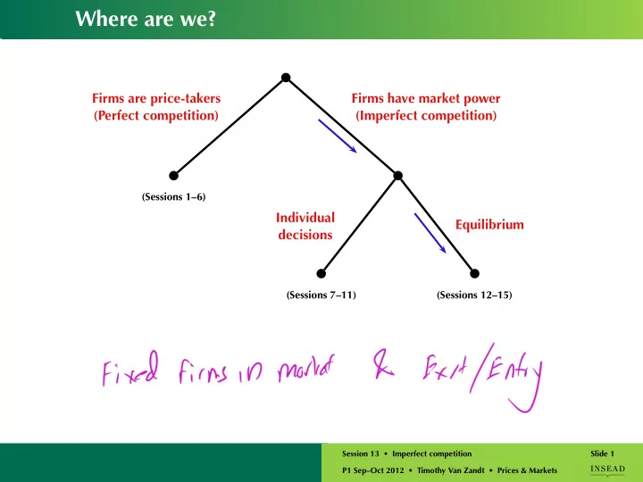
(Sessions 1–6)
Firms are price-takers (Perfect competition) Firms have market power (Imperfect competition)
(Sessions 7–11)
Individual decisions
(Sessions 12–15)
Equilibrium
Say: We did uniform pricing and price discrimination at individual level, but we only bring uniform pricing to equilibrium.
P1 Sep–Oct 2012 • Timothy Van Zandt • Prices & Markets Session 13 • Imperfect competition Slide 1