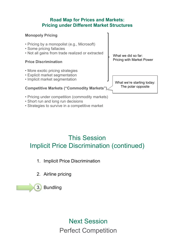
This Session Implicit Price Discrimination (continued) 1. Implicit - - PDF document

Monopoly Pricing

• Pricing by a monopolist (e.g., Microsoft)
• Some pricing fallacies
• Not all gains from trade realized or extracted

Price Discrimination

• More exotic pricing strategies
• Explicit market segmentation
• Implicit market segmentation

Competitive Markets (“Commodity Markets”)

• Pricing under competition (commodity markets)
• Short run and long run decisions
• Strategies to survive in a competitive market

Road Map for Prices and Markets: Pricing under Different Market Structures

What we’re starting today: The polar opposite What we did so far: Pricing with Market Power

This Session Implicit Price Discrimination (continued)

• 1. Implicit Price Discrimination
• 2. Airline pricing
• 3. Bundling

Next Session Perfect Competition

• Selling several goods in one bundle

! Hardware and software ! Software suites ! Sports/Concert tickets ! Auto accessories

Bundling

Exercise 6.6: Screening via Bundling

Pricing of the polo shirt and the dinner party at the Lebanese week. Highly segmented, with only three types of customers: Type of Customer Valuation Polo Shirt Dinner A $50 $5 B $40 $40 C $5 $50 A customer may buy either the polo shirt or the dinner.

– Benchmark: Perfect Price Discrimination – – No Bundling – – Pure Bundling – – Mixed Bundling – The Genius of Dell??

" Shoppers don't understand why retailers offer this kind of promotion when it's

no better for customers and no more profitable for stores than a half-price sale….

• Washington Post consumer columnist Margaret Webb Pressler

Hmmm…it is more profitable than a half-price sale!! Pizza: Valuation for 1st: $15.01; Valuation for 2nd: $5.01; MC = $2 BOGO at $20 Profit = 20 – 4 = 16 2 Pizzas for $10 each Profit = 10 – 2 = 8

What is this? Buy One Get One Free (BOGO)

This Session Implicit Price Discrimination

• 1. Implicit Price Discrimination
• 2. Airline pricing
• 3. Bundling

Next Session Perfect Competition

Bottom Line

Do not ignore the composition of your market! Marketing guru says: the right product for the right customer at the right price, Economist sage says: segment, differentiate, then segment some more!!

• 1. Find products where you can effectively prevent high-end consumers

from buying the low-end product

• 2. If you cant, implicitly segment the market – design a product line through

bundling, differentiation, versioning, inter-temporal pricing, damaging that achieves price discrimination

Prices and Markets

Session 9 Perfect Competition

• Prof. Amine Ouazad

Alusafs $2 billion question

1994: Alusaf wants to build a primary aluminum smelter

"

Capacity: 466 ktpy

"

Located at Richards bay, on the east coast of South Africa

"

Major bet: Capital expenditure close to 60% of Gencors net worth!! Feasibility study for this Hillside smelter was performed two years earlier

"

But aluminum prices plummeted to around $1,110 per ton ….as a result of the flow of Russian and other former eastern block countries Given that aluminum prices are at historic lows would you recommend dropping the Alusaf project?

This Session: Competitive Supply and Market Price

• 1. Alusaf’s $2 billion question
• 2. Perfect Competition
• 3. Primary Aluminum Market’s Supply
• 4. Demand Shocks

Next Session

Short-Run Costs and Prices

Perfect Competition

• Homogeneous product that is traded in a well-functioning transparent marketplace bringing

together lots of buyers and sellers easily ⇒ product sold at common “market price” determined by market-clearing condition: quantity supplied = quantity demanded

• Large number of small firms — no single producer can materially affect market price (at least

when industry was on flat portion of supply curve) ⇒ firms act as price takers

• Fragmented demand — no single buyer has significant “bargaining power” to affect the price
• Industries with these characteristics are close to the conditions of Perfect Competition.

Examples include:

• mining, such as copper
• primary metal fabrication, such as aluminum
• agricultural commodities
• certain types of commodity semi-conductors

Modeling Supply Decisions in Competitive Markets

Marginal conditions for optimal output (MR = MC): mc (q) = P → Supply curve s (P) is simply (inverse of) the marginal cost curve. P = MR s (P) d (P) Industry Firm mc (q) q Q $ $ q*

An Exercise

• There are 10 firms on a perfectly competitive market. Firms have

the same cost structure.

• c(Q) = 100 + 10Q + Q2
• mc(Q) =
• ac(Q) =
• Construct the supply curve of each firm, and the supply curve of

the market.

• A firm’s supply curve

si(P) =

• The market’s supply curve

s(P) =

• Shut down production if P <

10 20 30 40 50 60 70 80 5 10 15 20 25 30 35 mc(Q) ac(Q) avc(Q)

The Aggregate Supply Curve

1 2 3 4 5 6 7 8 9 10 11 12 13 14 15 2 4 6 8 10 12 14 16 18 20 Output Q $

s B (P) s A (P) s(P) = s A (P)+ s B (P)

d (P) P * Q *

Elasticity of Market Supply

Q P dP dQ Es = P Q E

s s

in change % in change % =

– Measuring responsiveness of supply to changes in price –

Point Elasticity

This Session: Competitive Supply and Market Price

• 1. Alusaf’s $2 billion question
• 2. Perfect Competition
• 3. Primary Aluminum Market’s Supply
• 4. Demand Shocks

Next Session

Short-Run Costs and Prices

Alusaf’s Hillside Project Seems like a simple business…

" Competitive Market – identical product; no tech. differences; price- takers " No room for fancy marketing strategies; nimble operational improvements " Profitability boils down to a simple equation price – average cost That cannot be that hard? " Need to understand:

• What determines prices?
• Which costs are relevant to Alusafs decision?
• What drives industry dynamics?

" For this, we need an economic model of what drives supply decisions and prices

Back to Alusaf: Cost (per ton) Analysis

Which costs are variable and which are fixed?

Smelter Sorocaba A Grand Baie Zaporozhye Country Brazil Canada Ukraine Company Other Alcan CIS Capacity (tpy) 122 180 100 Electricity usage (kWh/t) 15769 14215 17454 Electricity price ($/kWh) 0.005 0.005 0.008 Total electricity cost: 85.61 67.48 136.45 Alumina usage (t/t Al) 1.94 1.94 1.94 Alumina price ($/t Alumina) 111.83 179.39 146.58 Total alumina cost: 216.51 347.30 283.78 Other raw materials 156.19 95.66 58.28 Plant power and fuel 6.51 10.00 4.04 Consumables 79.28 42.16 67.31 Maintenance 30.13 52.93 32.57 Labor 150.40 149.85 17.27 Freight 43.43 39.09 48.86 General and administrative 57.66 66.27 72.16

Group 6, Section 6

Group 9, Section 7 Assuming variable cost includes all but labor, maintenance, plant power, and G&A

• Max. capacity

Supply of an Incumbent Firm: Constant MC

MC is vertical once capacity is reached

AC

• Min. AVC

SR shutdown

• Min. AC

LR shutdown

AVC = MC Short-run: P > MC = AVC then produce at capacity shut down in the short run if P<AVC Long-run: P > MC = AC then produce at capacity shut down in the long run if P<AC $

• Arrange firms by marginal cost in an ascending manner
• Table below shows the lowest 4 firms.

Firm Capacity Cumulative volume MC/ AVC Sorocaba 122 122 581 Grand Baie 180 302 591 Zaporozhye 100 402 594 Arvida 2 147 549 607

The World’s Supply Curve of Primary Aluminum

Section 7, Group 9

0. 0.00 00 500. 500.00 00 1000. 1000.00 00 1500. 1500.00 00 2000. 2000.00 00 2500. 2500.00 00 122 938.5 1800.5 3125.5 4082.2 5344.2 6537.5 7112.5 8646.5 9547.5 10233.5 11202.8 12065.8 12951.8 13625.3 14222 15375 16206 16830.5 17473 18069 18428 19129 19706 20027 20296.7 20884.7 Ou Output ('000 tons) Pri rice (per r ton)

Primary Aluminum Short Run Supply Curve

Market Demand Curve

In 1993, at a price of $1,110 " Actual production = 19,781 " Supply model predicts = 19,412 (cumulative capacity of plants whose P = 1,110 > MC) " Wow!! Anything else?? " Idle capacity of 950 thousand tpy in some European plants; low cost and should be operating at $1,110 " Subtract 950 from 19,412 to get Adjusted Supply = 18,462 Demand = 18,500

How does the model measure up to the data? Irrational Capacity: Incentives dont matter!

Is this the whole story? It cant be: Case says that inventories are accumulating fast, → supply > demand Explanation: Irrational Capacity which stays up and running regardless

• f pricing

" State-owned capacity that would not have operated under normal market incentives, but operates because decisions are driven by non-profit considerations " Add all state-owned capacity with average variable cost exceeding $1,110

How does the model measure up to the data?

Question: Given that Aluminum prices are at historical lows, should Alusaf drop the project? Answer depends on a more fundamental question: What is the relationship between current prices and long-run prices?

Actual demand 18,500 At a price of $1,110 the model predicts 19,412 Very close to actual production 19,781 Deduct 950 to adjust for idled European capacity 18,462 Add back 1,120 irrational capacity (difference builds up as inventories) 19,582

This Session: Competitive Supply and Market Price

• 1. Perfect Competition
• 2. Alusaf’s $2 billion question
• 3. Primary Aluminum Market’s Supply
• 4. Demand Shocks and Price Effects

Are we missing something?

Next Session

Short-Run Costs and Prices

0. 0.00 00 500. 500.00 00 1000. 1000.00 00 1500. 1500.00 00 2000. 2000.00 00 2500. 2500.00 00 5000 10000 15000 20000 25000 Ou Output ('000 tons) Pri rice (per r ton)

Short Run Demand Curve (inelastic)

Aluminum in 1992: Introduction of new capacity can lead to catastrophic collapse in prices

New Capacity

Collapse when: a) Demand highly inelastic; b) Initial equilibrium on steep segment of supply curve

0. 0.00 00 500. 500.00 00 1000. 1000.00 00 1500. 1500.00 00 2000. 2000.00 00 2500. 2500.00 00 5000 10000 15000 20000 25000 Ou Output ('000 tons) Pri rice (per r ton)

It All Depends on Relative Demand and Supply

But if supply intersects demand on the flat segment of the supply curve then… Demand and supply can vary by a significant amount without big prices changes

Elasticity of Market Supply

Q P dP dQ Es = P Q E

s s

in change % in change % =

– Measuring responsiveness of supply to changes in price –

Point Elasticity Lessons for a smart investor??

“We think gold and platinum are an outright buy at present levels as both metals have very low supply elasticity and are key beneficiaries

• f loose monetary policy” UBS Gold Outlook

2013 "In view of the expected high demand, pressure on real estate prices may continue. Such developments can easily generate bubbles in the real estate market because of problems in the elasticity of supply.”

• - Rakesh Mohan, Deputy

Governor, Bank of India, Dec. 2007

This Session: Competitive Supply and Market Price

• 1. Perfect Competition
• 2. Alusaf’s $2 billion question
• 3. Primary Aluminum Market’s Supply
• 4. Demand Shocks

Next Session

Short-Run Costs and Prices

Take Away Point from Alusaf

So what is the relationship between current prices and long-run profitability?

" Quick answer: NONE!! " Firms make mistakes and can lose profits if they misinterpret short-run fluctuations and trends " KEY IMPLICATIONS: # It is very dangerous to be either overly optimistic or overly pessimistic about a commodity market opportunity based on just observing short- run trends # You need to forecast long run prices (next session)

Wrap up

• A perfectly competitive market has:
• A large number of small players, i.e. fragmented supply and demand.
• A homogeneous product.
• In a perfectly competitive market, firms are price-takers, and MR=p. Firms produce

quantity Q such that p = MC. The firm’s supply curve is the inverse of the marginal cost curve.

• Construct the market’s supply curve by adding the firms’ supply curves horizontally.

Use the market’s supply curve to forecast the effect of demand shocks on the market’s price.

• The effect of demand shocks on the market price are larger when supply is inelastic.
• At this point, is our analysis complete???
• The decision of Alusaf depends on the forecast of the price of aluminum and the

average cost of production.

Next session : Short Run Costs and Prices

• Answer this: Should Alusaf invest $2b in the Hillside Plant?
• Reading:
• Course Guide Chapter 11.
• Read “Reading the Course Guide” !!
• Chipmakers signal second dip, Financial Times, October 7,

2010.