
SLIDE 1
1
(c) 2003 Thomas G. Dietterich 1
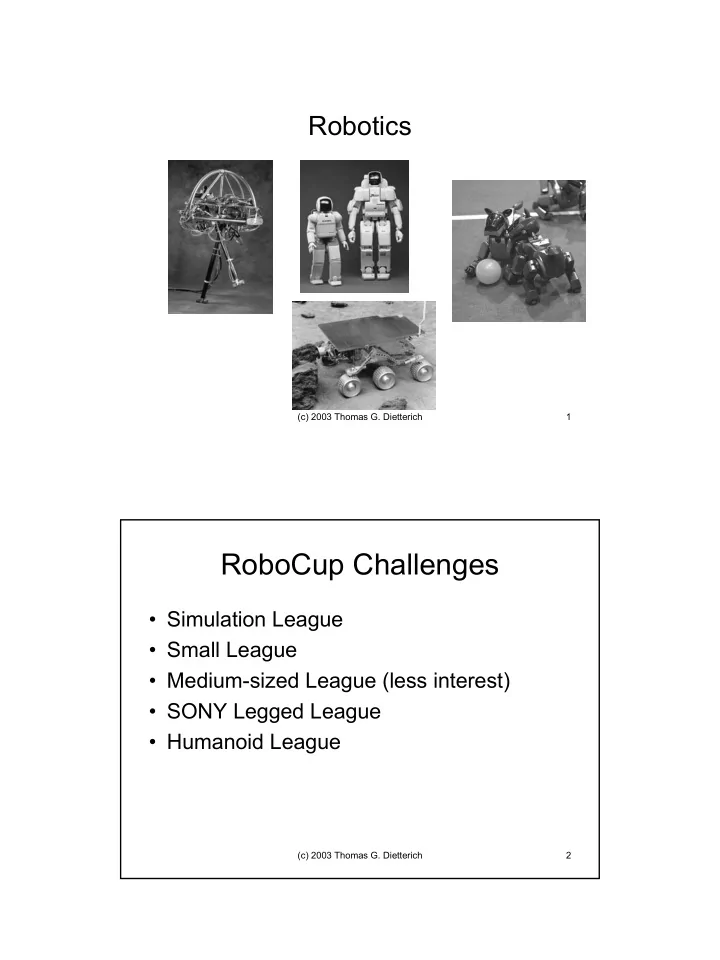
Robotics
(c) 2003 Thomas G. Dietterich 2
RoboCup Challenges
- Simulation League
- Small League
- Medium-sized League (less interest)
- SONY Legged League
- Humanoid League