Connectivity of random irrigation networks Nicolas Broutin, Luc - - PowerPoint PPT Presentation

Connectivity of random irrigation networks

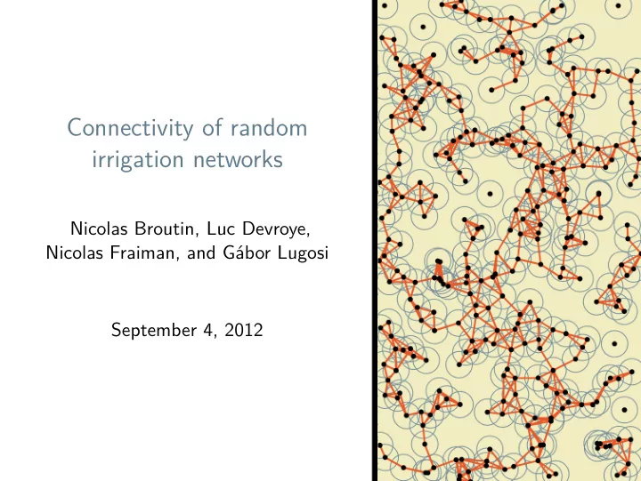
Nicolas Broutin, Luc Devroye, Nicolas Fraiman, and G´ abor Lugosi September 4, 2012

Irrigation graph

Start with a connected graph on n vertices. An irrigation subgraph is obtained when that each vertex selects c neighbors at random (without replacement). We consider the case when the underlying graph is a random geometric graph such that the vertices are X1 Xn be i.i.d. uniform on 0 1 d and Xi Xj iff Xi Xj r. Such graphs are also called bluetooth graphs. They are locally sparsified random geometric graphs. The model was introduced by Ferraguto, Mambrini, Panconesi, and Petrioli ”A new approach to device discovery and scatternet formation in bluetooth networks” (2004). Main question: How large does c need to be for G n r c to be connected?

Irrigation graph

Start with a connected graph on n vertices. An irrigation subgraph is obtained when that each vertex selects c neighbors at random (without replacement). We consider the case when the underlying graph is a random geometric graph such that the vertices are X1 Xn be i.i.d. uniform on 0 1 d and Xi Xj iff Xi Xj r. Such graphs are also called bluetooth graphs. They are locally sparsified random geometric graphs. The model was introduced by Ferraguto, Mambrini, Panconesi, and Petrioli ”A new approach to device discovery and scatternet formation in bluetooth networks” (2004). Main question: How large does c need to be for G n r c to be connected?

Irrigation graph

Start with a connected graph on n vertices. An irrigation subgraph is obtained when that each vertex selects c neighbors at random (without replacement). We consider the case when the underlying graph is a random geometric graph such that the vertices are X1,...,Xn be i.i.d. uniform on [0,1]d and Xi ∼ Xj iff Xi −Xj < r. Such graphs are also called bluetooth graphs. They are locally sparsified random geometric graphs. The model was introduced by Ferraguto, Mambrini, Panconesi, and Petrioli ”A new approach to device discovery and scatternet formation in bluetooth networks” (2004). Main question: How large does c need to be for G n r c to be connected?

Irrigation graph

Start with a connected graph on n vertices. An irrigation subgraph is obtained when that each vertex selects c neighbors at random (without replacement). We consider the case when the underlying graph is a random geometric graph such that the vertices are X1,...,Xn be i.i.d. uniform on [0,1]d and Xi ∼ Xj iff Xi −Xj < r. Such graphs are also called bluetooth graphs. They are locally sparsified random geometric graphs. The model was introduced by Ferraguto, Mambrini, Panconesi, and Petrioli ”A new approach to device discovery and scatternet formation in bluetooth networks” (2004). Main question: How large does c need to be for G n r c to be connected?

Irrigation graph

Start with a connected graph on n vertices. An irrigation subgraph is obtained when that each vertex selects c neighbors at random (without replacement). We consider the case when the underlying graph is a random geometric graph such that the vertices are X1,...,Xn be i.i.d. uniform on [0,1]d and Xi ∼ Xj iff Xi −Xj < r. Such graphs are also called bluetooth graphs. They are locally sparsified random geometric graphs. The model was introduced by Ferraguto, Mambrini, Panconesi, and Petrioli ”A new approach to device discovery and scatternet formation in bluetooth networks” (2004). Main question: How large does c need to be for G n r c to be connected?

Irrigation graph

Start with a connected graph on n vertices. An irrigation subgraph is obtained when that each vertex selects c neighbors at random (without replacement). We consider the case when the underlying graph is a random geometric graph such that the vertices are X1,...,Xn be i.i.d. uniform on [0,1]d and Xi ∼ Xj iff Xi −Xj < r. Such graphs are also called bluetooth graphs. They are locally sparsified random geometric graphs. The model was introduced by Ferraguto, Mambrini, Panconesi, and Petrioli ”A new approach to device discovery and scatternet formation in bluetooth networks” (2004). Main question: How large does c need to be for G(n,r,c) to be connected?

Irrigation graph

• G(n,r,c) is a subgraph of a random geometric graph G(n,r),

so we need G(n,r) to be connected. Penrose (1997) showed that 0, G n r is connected whp if r 1 rt where rt

d

logn n

1 d

and

d

2 2dVolB 0 1

1 d

We only consider values of r above this level.

Irrigation graph

• G(n,r,c) is a subgraph of a random geometric graph G(n,r),

so we need G(n,r) to be connected.

• Penrose (1997) showed that ∀ε > 0, G(n,r) is connected whp if

r ≥ (1+ε)rt where rt = θd

(logn

n

)1/d

and

θd =

2 (2dVolB(0,1))1/d . We only consider values of r above this level.

Irrigation graph

Irrigation graph

Irrigation graph

Previous results

Theorem (Fenner and Frieze, 1982)

For r = ∞, the graph G(n,r,2) (the random 2-out graph) is connected whp.

Theorem (Dubhashi, Johansson, Haggstrom, Panconesi, Sozio, 2007)

For constant r the graph G n r 2 is connected whp.

Theorem (Crescenzi, Nocentini, Pietracaprina, Pucci, 2009)

In dimension d 2, such that if r logn n and c log 1 r then G n r c is connected whp.

Previous results

Theorem (Fenner and Frieze, 1982)

For r = ∞, the graph G(n,r,2) (the random 2-out graph) is connected whp.

Theorem (Dubhashi, Johansson, H¨

aggstr¨

• m, Panconesi, Sozio, 2007)

For constant r the graph G(n,r,2) is connected whp.

Theorem (Crescenzi, Nocentini, Pietracaprina, Pucci, 2009)

In dimension d 2, such that if r logn n and c log 1 r then G n r c is connected whp.

Previous results

Theorem (Fenner and Frieze, 1982)

For r = ∞, the graph G(n,r,2) (the random 2-out graph) is connected whp.

Theorem (Dubhashi, Johansson, H¨

aggstr¨

• m, Panconesi, Sozio, 2007)

For constant r the graph G(n,r,2) is connected whp.

Theorem (Crescenzi, Nocentini, Pietracaprina, Pucci, 2009)

In dimension d = 2, ∃ α,β such that if r ≥ α

√

logn n and c ≥ βlog(1/r), then G(n,r,c) is connected whp.

Main result

Theorem

There exists a constant γ∗ > 0 such that for all γ ≥ γ∗ and ε ∈ (0,1), if r ∼ γ

(logn

n

)1/d

and ct =

√

2logn loglogn, then if c 1 ct then G n r c is connected whp. if c 1 ct then G n r c is disconnected whp. ct does not depend on

• r d.

Main result

Theorem

There exists a constant γ∗ > 0 such that for all γ ≥ γ∗ and ε ∈ (0,1), if r ∼ γ

(logn

n

)1/d

and ct =

√

2logn loglogn, then

• if c ≥ (1+ε)ct then G(n,r,c) is connected whp.
• if c ≤ (1−ε)ct then G(n,r,c) is disconnected whp.

ct does not depend on

• r d.

Main result

Theorem

There exists a constant γ∗ > 0 such that for all γ ≥ γ∗ and ε ∈ (0,1), if r ∼ γ

(logn

n

)1/d

and ct =

√

2logn loglogn, then

• if c ≥ (1+ε)ct then G(n,r,c) is connected whp.
• if c ≤ (1−ε)ct then G(n,r,c) is disconnected whp.

ct does not depend on γ or d.

Below the threshold

Theorem

Let γ ≥ γ∗ and ε ∈ (0,1). If r = γ

(logn

n

)1/d and

c ≤ (1−ε)ct then G(n,r,c) is disconnected whp. The smallest possible components are cliques of size c 1.

Below the threshold

Theorem

Let γ ≥ γ∗ and ε ∈ (0,1). If r = γ

(logn

n

)1/d and

c ≤ (1−ε)ct then G(n,r,c) is disconnected whp.

• The smallest possible

components are cliques of size c+1.

Below the threshold

Theorem

Let γ ≥ γ∗ and ε ∈ (0,1). If r = γ

(logn

n

)1/d and

c ≤ (1−ε)ct then G(n,r,c) is disconnected whp.

• The smallest possible

components are cliques of size c+1.

Isolated (c+1)-cliques

• We show that there exists an isolated (c+1)-clique whp.

Let be the random family of subsets of 1 n given by Q 1 n Q c 1 Xi Xj r i j Q Let I Q be the indicator of the event that Q is an isolated clique. Then N

Q

I Q is the number of isolated c 1 -cliques.

Isolated (c+1)-cliques

• We show that there exists an isolated (c+1)-clique whp.
• Let F be the random family of subsets of {1,...,n} given by

F = {

Q ⊂

{1,...,n } : |Q| = c+1, Xi −Xj < r ∀i,j ∈ Q } .

Let I Q be the indicator of the event that Q is an isolated clique. Then N

Q

I Q is the number of isolated c 1 -cliques.

Isolated (c+1)-cliques

• We show that there exists an isolated (c+1)-clique whp.
• Let F be the random family of subsets of {1,...,n} given by

F = {

Q ⊂

{1,...,n } : |Q| = c+1, Xi −Xj < r ∀i,j ∈ Q } .

• Let I(Q) be the indicator of the event that Q is an isolated clique.

Then N = ∑

Q∈F I(Q) is the number of isolated (c+1)-cliques.

Isolated (c+1)-cliques

• We need some regularity on the uniformly distributed points.

For every 1 ≤ j ≤ n

αnr2 < # {i : Xi ∈ B(Xj,r) } < βnr2.

Let D be the event described above. We use the second-moment method and prove that P N1D E N1D

2

E N21D 1

Isolated (c+1)-cliques

• We need some regularity on the uniformly distributed points.

For every 1 ≤ j ≤ n

αnr2 < # {i : Xi ∈ B(Xj,r) } < βnr2.

• Let D be the event described above. We use the second-moment

method and prove that P

{N1D > 0 } ≥ E {N1D }2

E

{

N21D

} → 1.

Above the threshold

Theorem

Let γ ≥ γ∗ and ε ∈ (0,1). If r = γ

(logn

n

)1/d and

c ≥ (1+ε)ct then G(n,r,c) is connected whp.

Gridding and percolation

We tile the unit square [0,1]2 into cells of side length r. Two cells are connected if they are adjacent and there is an edge between one vertex of each cell. Two cells are

• connected if they share at least a corner and there is

an edge between one vertex of each cell. A cell is colored black if all the vertices in it are connected to each

• ther without using an edge that leaves the cell. The other cells are

initially colored white.

Gridding and percolation

We tile the unit square [0,1]2 into cells of side length r.

• Two cells are connected if they are adjacent and there is an edge

between one vertex of each cell. Two cells are

• connected if they share at least a corner and there is

an edge between one vertex of each cell. A cell is colored black if all the vertices in it are connected to each

• ther without using an edge that leaves the cell. The other cells are

initially colored white.

Gridding and percolation

We tile the unit square [0,1]2 into cells of side length r.

• Two cells are connected if they are adjacent and there is an edge

between one vertex of each cell.

• Two cells are ∗-connected if they share at least a corner and there is

an edge between one vertex of each cell. A cell is colored black if all the vertices in it are connected to each

• ther without using an edge that leaves the cell. The other cells are

initially colored white.

Gridding and percolation

We tile the unit square [0,1]2 into cells of side length r.

• Two cells are connected if they are adjacent and there is an edge

between one vertex of each cell.

• Two cells are ∗-connected if they share at least a corner and there is

an edge between one vertex of each cell.

• A cell is colored black if all the vertices in it are connected to each
• ther without using an edge that leaves the cell. The other cells are

initially colored white.

Gridding and percolation

The following properties hold whp:

• 1. Every cell in the grid contains at most

logn vertices for some .

• 2. Every cell in the grid connects to its adjacent cells.
• 3. Every
• connected component of white cells has size at most

q 2 logn 2 3.

• 4. Every connected component of G has size at least s

exp logn 1 3 .

Gridding and percolation

The following properties hold whp:

• 1. Every cell in the grid contains at most λlogn vertices for some

λ = λ(γ).

• 2. Every cell in the grid connects to its adjacent cells.
• 3. Every
• connected component of white cells has size at most

q 2 logn 2 3.

• 4. Every connected component of G has size at least s

exp logn 1 3 .

Gridding and percolation

The following properties hold whp:

• 1. Every cell in the grid contains at most λlogn vertices for some

λ = λ(γ).

• 2. Every cell in the grid connects to its adjacent cells.
• 3. Every
• connected component of white cells has size at most

q 2 logn 2 3.

• 4. Every connected component of G has size at least s

exp logn 1 3 .

Gridding and percolation

The following properties hold whp:

• 1. Every cell in the grid contains at most λlogn vertices for some

λ = λ(γ).

• 2. Every cell in the grid connects to its adjacent cells.
• 3. Every ∗-connected component of white cells has size at most

q = 2(logn)2/3.

• 4. Every connected component of G has size at least s

exp logn 1 3 .

Gridding and percolation

The following properties hold whp:

• 1. Every cell in the grid contains at most λlogn vertices for some

λ = λ(γ).

• 2. Every cell in the grid connects to its adjacent cells.
• 3. Every ∗-connected component of white cells has size at most

q = 2(logn)2/3.

• 4. Every connected component of G has size at least s = exp((logn)1/3).

The four properties

• 1. Every cell in the grid contains at most λlogn vertices.

Concentration of number of points in cells. E C nr2 logn .

The four properties

• 1. Every cell in the grid contains at most λlogn vertices.
• Concentration of number of points in cells.
• E

{#C } = Θ(nr2) = Θ(logn).

The four properties

• 2. Every cell in the grid connects to its adjacent cells.

Subdivide the cell and find an edge bewteen two squares in the border.

The four properties

• 2. Every cell in the grid connects to its adjacent cells.
• Subdivide the cell and find

an edge bewteen two squares in the border.

The four properties

• 3. Every ∗-connected component of white cells has size at most

q = 2(logn)2/3.

• connected comp. of size k

n 8e k. It suffices to show that P Cell is white p exp logn 2 3 . If k q then n 8e kpk 0.

The four properties

• 3. Every ∗-connected component of white cells has size at most

q = 2(logn)2/3.

• #

{ ∗-connected comp. of size k } ≤ n(8e)k.

It suffices to show that P Cell is white p exp logn 2 3 . If k q then n 8e kpk 0.

The four properties

• 3. Every ∗-connected component of white cells has size at most

q = 2(logn)2/3.

• #

{ ∗-connected comp. of size k } ≤ n(8e)k.

• It suffices to show that

P

{Cell is white } ≤ p = exp(−(logn)2/3).

If k q then n 8e kpk 0.

The four properties

• 3. Every ∗-connected component of white cells has size at most

q = 2(logn)2/3.

• #

{ ∗-connected comp. of size k } ≤ n(8e)k.

• It suffices to show that

P

{Cell is white } ≤ p = exp(−(logn)2/3).

If k q then n 8e kpk 0.

The four properties

• 3. Every ∗-connected component of white cells has size at most

q = 2(logn)2/3.

• #

{ ∗-connected comp. of size k } ≤ n(8e)k.

• It suffices to show that

P

{Cell is white } ≤ p = exp(−(logn)2/3).

If k q then n 8e kpk 0.

The four properties

• 3. Every ∗-connected component of white cells has size at most

q = 2(logn)2/3.

• #

{ ∗-connected comp. of size k } ≤ n(8e)k.

• It suffices to show that

P

{Cell is white } ≤ p = exp(−(logn)2/3).

If k q then n 8e kpk 0.

The four properties

• 3. Every ∗-connected component of white cells has size at most

q = 2(logn)2/3.

• #

{ ∗-connected comp. of size k } ≤ n(8e)k.

• It suffices to show that

P

{Cell is white } ≤ p = exp(−(logn)2/3).

• If k > q then n(8e)kpk → 0.

The four properties

• 4. Every connected component of G has size at least s = exp((logn)1/3).

Save 2 ct edge choices. No small components with 1 2 ct choices. Use extra edges iteratively to double the size of components.

The four properties

• 4. Every connected component of G has size at least s = exp((logn)1/3).
• Save (ε/2)ct edge choices.

No small components with 1 2 ct choices. Use extra edges iteratively to double the size of components.

The four properties

• 4. Every connected component of G has size at least s = exp((logn)1/3).
• Save (ε/2)ct edge choices.
• No small components with (1+ε/2)ct choices.

Use extra edges iteratively to double the size of components.

The four properties

• 4. Every connected component of G has size at least s = exp((logn)1/3).
• Save (ε/2)ct edge choices.
• No small components with (1+ε/2)ct choices.
• Use extra edges iteratively to double the size of components.

Gridding and percolation

• 1. Every cell in the grid contains at most λlogn vertices.
• 2. Every cell in the grid connects to its adjacent cells.
• 3. Every ∗-connected component of white cells has size at most q cells.
• 4. Every connected component of G has size at least s.

If all properties hold, then the whole graph is connected.

Everything is connected

• Black connector: There exists a connected component of black cells

that links two opposite sides of [0,1]2. Black giant: Black components of size less than 1 r are now recolored

• gray. All remaining black cells are connected. The corresponding

vertices of G belong to the same connected component. Connectivity: Each vertex connects to at least one vertex of the black giant.

Everything is connected

• Black connector: There exists a connected component of black cells

that links two opposite sides of [0,1]2.

• Black giant: Black components of size less than 1/r are now recolored
• gray. All remaining black cells are connected. The corresponding

vertices of G belong to the same connected component.

• Connectivity: Each vertex connects to at least one vertex of the black

giant.

Everything is connected

K K′

Spanning ratio and diameter

An important feature of a geometric graph is the spanning ratio sup

i,j

dist(Xi,Xj)

Xi −Xj

where dist(Xi,Xj) is the shortest (Euclidean) distance of Xi and Xj over the edges of the graph. Ideally, this should be small. Unfortunately, this can be large if Xi and Xj are very close. However, for c slightly larger than critical, we have

Theorem

K 0 such that if , r

logn n 1 d and c

logn then sup

i j Xi Xj r

dist Xi Xj Xi Xj K whp.

Spanning ratio and diameter

An important feature of a geometric graph is the spanning ratio sup

i,j

dist(Xi,Xj)

Xi −Xj

where dist(Xi,Xj) is the shortest (Euclidean) distance of Xi and Xj over the edges of the graph. Ideally, this should be small. Unfortunately, this can be large if Xi and Xj are very close. However, for c slightly larger than critical, we have

Theorem

K 0 such that if , r

logn n 1 d and c

logn then sup

i j Xi Xj r

dist Xi Xj Xi Xj K whp.

Spanning ratio and diameter

An important feature of a geometric graph is the spanning ratio sup

i,j

dist(Xi,Xj)

Xi −Xj

where dist(Xi,Xj) is the shortest (Euclidean) distance of Xi and Xj over the edges of the graph. Ideally, this should be small. Unfortunately, this can be large if Xi and Xj are very close. However, for c slightly larger than critical, we have

Theorem

∃K,µ > 0 such that if γ > γ∗,

r = γ

(logn

n

)1/d and c ≥ µ √

logn then sup

i,j:Xi−Xj>r

dist(Xi,Xj)

Xi −Xj ≤ K,

whp.

Spanning ratio and diameter

This implies that the diameter of G satisfies diam(G) ≤ K

• d/r. This is
• ptimal, up to a constant factor.

Idea of the proof: Partition the unit cube into a grid of cells of side length 1 3 1 r

1.

With high probability, any two points i and j, such that Xi and Xj fall in the same cell, are connected by a path of length at most five. On the other hand, with high probability, any two neighboring cells contain two points, one in each cell, that are connected by an edge of Sn.

Spanning ratio and diameter

This implies that the diameter of G satisfies diam(G) ≤ K

• d/r. This is
• ptimal, up to a constant factor.

Idea of the proof: Partition the unit cube into a grid of cells of side length

ℓ = (1/3) ⌊1/r ⌋−1.

With high probability, any two points i and j, such that Xi and Xj fall in the same cell, are connected by a path of length at most five. On the other hand, with high probability, any two neighboring cells contain two points, one in each cell, that are connected by an edge of Sn.

Supercritical radii

The proof of disconnectedness may be generalized easily for the entire range of values of r.

Theorem

Let 0 1 and 1 be such that

logn n 1 d

r d, lognrd loglogn and c 1 1 2 logn lognrd Then G n r c is disconnected whp. In particular, take r n

1

• d. Then for c

1 (constant) the graph is disconnected.

Supercritical radii

The proof of disconnectedness may be generalized easily for the entire range of values of r.

Theorem

Let

ε ∈ (0,1)

and

λ ∈ [1,∞]

be such that

γ∗ (logn

n

)1/d < r <

• d,

lognrd loglogn → λ and c ≤ (1−ε)

√( λ λ−1/2 ) logn

lognrd . Then G(n,r,c) is disconnected whp. In particular, take r n

1

• d. Then for c

1 (constant) the graph is disconnected.

Supercritical radii

The proof of disconnectedness may be generalized easily for the entire range of values of r.

Theorem

Let

ε ∈ (0,1)

and

λ ∈ [1,∞]

be such that

γ∗ (logn

n

)1/d < r <

• d,

lognrd loglogn → λ and c ≤ (1−ε)

√( λ λ−1/2 ) logn

lognrd . Then G(n,r,c) is disconnected whp. In particular, take r ∼ n−(1−δ)/d. Then for c ≤ (1−ǫ)/

• δ (constant) the

graph is disconnected.

Supercritical r, constant c

We can show that the lower bound is not far from the truth: when r ∼ n−(1−δ)/d, constant c is sufficient for connectivity. c =

√

5/δ+c(d) is sufficient for connectivity. The irrigation graph is genuinely sparse.

Supercritical r, constant c

Theorem

Let δ ∈ (0,1), γ > 0. Suppose that rn ∼ γn−(1−δ)/d. There exists a constant c = c(δ,d) such that G is connected whp. One may take c = c1 +c2 +c3 +1, where c1 = ⌈

√

5/(δ−δ2)⌉ , and c2,c3 depend on d only.

Supercritical r, constant c

Sketch of proof:

• First show that X1,...,Xn are sufficiently regular whp. Once the Xi are

fixed, all randomness comes from the edge choices. We add edges in four phases. In the first we start from X1, and using c1 choices of each vertex, we go for

2logc1 n generations. There exists a

cube in the grid that contains a connected component of size nconst. 2. Second, we add c2 new connections to each vertex in the component. At least one of the grid cells has a positive fraction of its points in a connected component. Third, using c3 new connections of each vertex, we obtain a connected component that contains a constant fraction of the points in every cell of the grid, whp. Finally, add just one more connection per vertex so that the entire graph becomes connected.

Supercritical r, constant c

Sketch of proof:

• First show that X1,...,Xn are sufficiently regular whp. Once the Xi are

fixed, all randomness comes from the edge choices.

• We add edges in four phases. In the first we start from X1, and using c1

choices of each vertex, we go for δ2logc1 n generations. There exists a cube in the grid that contains a connected component of size nconst.δ2. Second, we add c2 new connections to each vertex in the component. At least one of the grid cells has a positive fraction of its points in a connected component. Third, using c3 new connections of each vertex, we obtain a connected component that contains a constant fraction of the points in every cell of the grid, whp. Finally, add just one more connection per vertex so that the entire graph becomes connected.

Supercritical r, constant c

Sketch of proof:

• First show that X1,...,Xn are sufficiently regular whp. Once the Xi are

fixed, all randomness comes from the edge choices.

• We add edges in four phases. In the first we start from X1, and using c1

choices of each vertex, we go for δ2logc1 n generations. There exists a cube in the grid that contains a connected component of size nconst.δ2.

• Second, we add c2 new connections to each vertex in the component. At

least one of the grid cells has a positive fraction of its points in a connected component. Third, using c3 new connections of each vertex, we obtain a connected component that contains a constant fraction of the points in every cell of the grid, whp. Finally, add just one more connection per vertex so that the entire graph becomes connected.

Supercritical r, constant c

Sketch of proof:

• First show that X1,...,Xn are sufficiently regular whp. Once the Xi are

fixed, all randomness comes from the edge choices.

• We add edges in four phases. In the first we start from X1, and using c1

choices of each vertex, we go for δ2logc1 n generations. There exists a cube in the grid that contains a connected component of size nconst.δ2.

• Second, we add c2 new connections to each vertex in the component. At

least one of the grid cells has a positive fraction of its points in a connected component.

• Third, using c3 new connections of each vertex, we obtain a connected

component that contains a constant fraction of the points in every cell of the grid, whp. Finally, add just one more connection per vertex so that the entire graph becomes connected.

Supercritical r, constant c

Sketch of proof:

• First show that X1,...,Xn are sufficiently regular whp. Once the Xi are

fixed, all randomness comes from the edge choices.

• We add edges in four phases. In the first we start from X1, and using c1

choices of each vertex, we go for δ2logc1 n generations. There exists a cube in the grid that contains a connected component of size nconst.δ2.

• Second, we add c2 new connections to each vertex in the component. At

least one of the grid cells has a positive fraction of its points in a connected component.

• Third, using c3 new connections of each vertex, we obtain a connected

component that contains a constant fraction of the points in every cell of the grid, whp.

• Finally, add just one more connection per vertex so that the entire graph

becomes connected.

Thank you