Quantum optics and information with trapped ions Introduction to - - PowerPoint PPT Presentation

• Introduction to ion trapping and cooling
• Trapped ions as qubits for quantum computing and simulation
• Rydberg excitations for fast entangling operations
• Quantum thermodynamics, Kibble Zureck law, and heat

engines

• Implanting single ions for a solid state quantum device

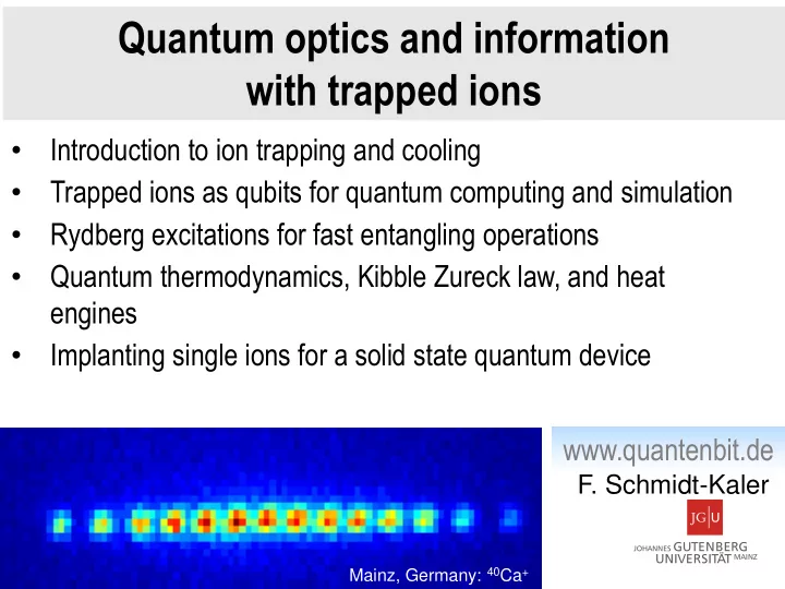
www.quantenbit.de

Quantum optics and information with trapped ions

• F. Schmidt-Kaler

Mainz, Germany: 40Ca+

Ion Gallery

Boulder, USA: Hg+ Aarhus, Denmark: 40Ca+ (red) and 24Mg+ (blue) Oxford, England: 40Ca+ coherent breathing motion of a 7-ion linear crystal Innsbruck, Austria: 40Ca+

Why using ions?

• Ions in Paul traps were the first sample with which laser cooling was

demonstrated and quite some Nobel prizes involve laser cooling…

• A single laser cooled ion still represents one of the best understood objects for

fundamental investigations of the interaction between matter and radiation

• Experiments with single ions spurred the development of similar methods with

neutral atoms

• Particular advantages of ions are that they are
• confined to a very small spatial region (dx<l)
• controlled and measured at will for experimental times of days
• Ideal test ground for fundamental quantum optical experiments
• Further applications for
• precision measurements
• cavity QED
• optical clocks
• quantum computing
• thermodynamics with small systems
• quantum phase transitions

Paul trap in 3D Linear Paul trap micro traps: segmented linear trap planar segmented trap Eigenmodes of a linear ion crystal Stability of a linear crystal planar ion crystals non-harmonic contributions Micromotion

Introduction to ion trapping

Traditional Paul trap Modern segmented micro Paul trap

Dynamic confinement in Paul trap

Invention of the Paul trap

Wolfgang Paul (Nobel prize 1989)

Binding in three dimensions

Electrical quadrupole potential Binding force for charge Q leads to a harmonic binding:

no static trapping in 3 dimensions

Laplace equation requires Ion confinement requires a focusing force in 3 dimensions, but such that at least one of the coefficients is negative, e.g. binding in x- and y-direction but anti-binding in z-direction !

trap size:

Dynamical trapping: Paul‘s idea

time depending potential with leads to the equation of motion for a particle with charge Q and mass m takes the standard form of the Mathieu equation (linear differential equ. with time depending cofficients) with substitutions radial and axial trap radius

Mechanical Paul trap

Rotating saddle Stable confinement

• f a ball in the

rotating potential X-direction Y-direction

Regions of stability

time-periodic diff. equation leads to Floquet Ansatz If the exponent µ is purely real, the motion is bound, if µ has some imaginary part x is exponantially growing and the motion is unstable. The parameters a and q determine if the motion is stable or not. Find solution analytically (complicated) or numerically: a=0, q =0.1 a=0, q =0.2

time time excursion excursion

a=0, q =0.3 a=0, q =0.4

time time excursion excursion

a=0, q =0.5 a=0, q =0.6

time time excursion excursion

a=0, q =0.7 a=0, q =0.8

time time excursion excursion

a=0, q =0.9 a=0, q =1.0

time time excursion excursion 6 1019

• 3 1019

unstable

time position in trap micromotion

1D-solution of Mathieu equation single Aluminium dust particle in trap

Two oscillation frequencies

slow frequency: Harmonic secular motion, frequency w increases with increasing q fast frequency: Micromotion with frequency W Ion is shaken with the RF drive frequency (disappears at trap center) Lissajous figure

3-Dim. Paul trap stability diagram

for a << q << 1 exist approximate solutions The 3D harmonic motion with frequency wi can be interpreted, approximated, as being caused by a pseudo-potential Y leads to a quantized harmonic oscillator PP approx. : RMP 75, 281 (2003), NJP 14, 093023 (2012), PRL 109, 263003 (2012)

Real 3-Dim. Paul traps

ideal 3-Dim. Paul trap with equi-potental surfaces formed by copper electrodes endcap electrodes at distance ideal surfaces: but non-ideal surfaces do trap also well: rring ~ 1.2mm

• A. Mundt, Innsbruck

ideal 3 dim. Paul trap with equi-potental surfaces formed by copper electrodes non-ideal surfaces rring ~ 1.2mm numerical calculation

• f equipotental lines

similar potential near the center

Real 3-Dim. Paul traps

RMP 82, 2609 (2010)

x y

2-Dim. Paul mass filter stability diagram

time depending potential with dynamical confinement in the x- y-plane with substitutions radial trap radius

2-Dim. Paul mass filter stability diagram

x y

A Linear Paul trap

plug the ends of a mass filter by positive electrodes: mass filter blade design side view RF RF 0V 0V Uend Uend numerically calculate the axial electric potential, fit parabula into the potential and get the axial trap frequency with k geometry factor

z0

Numerical tools: RMP 82, 2609 (2010)

Innsbruck design of linear ion trap

1.0mm 5mm

MHz 5 

radial

w MHz 2 7 .  

axial

w

Blade design

eV depth trap 

• F. Schmidt-Kaler, et al.,
• Appl. Phys. B 77, 789 (2003).

Ion crystals: Equilibrium positions and eigenmodes

Equilibrium positions in the axial potential

z-axis

mutual ion repulsion trap potential find equilibrium positions x0: ions oscillate with q(t) arround condition for equilibrium: dimensionless positions with length scale

• D. James, Appl. Phys.

B 66, 181 (1998)

Equilibrium positions in the axial potential

numerical solution (Mathematica), e.g. N=5 ions equilibrium positions set of N equations for um

• 1.74
• 0.82

0 +0.82 +1.74 force of the trap potential Coulomb force

• f all ions from left side

Coulomb force

• f all ions from left side

• 40
• 30
• 20
• 10

10 20 30 40 1 2 3 4 5 6 7 8 9 10 Number of Ions z-position (µm)

Linear crystal equilibrium positions

equilibrium positions are not equally spaced

• H. C. Nägerl et al.,
• Appl. Phys. B 66, 603 (1998)

theory experiment

minimum inter-ion distance:

Eigenmodes and Eigenfrequencies

Lagrangian of the axial ion motion:

m,n=1 m=1 N N

describes small excursions arround equilibrium positions with and

N m,n=1 m=1 N N

• D. James, Appl. Phys.

B 66, 181 (1998) linearized Coulomb interaction leads to Eigenmodes, but the next term in Tailor expansion leads to mode coupling, which is however very small.

• C. Marquet, et al.,
• Appl. Phys. B 76, 199

(2003)

Eigenmodes and Eigenfrequencies

Matrix, to diagonize numerical solution (Mathematica), e.g. N=4 ions Eigenvectors Eigenvalues for the radial modes: Market et al., Appl. Phys. B76, (2003) 199

depends on N

pictorial

does not

time position

Center of mass mode breathing mode

Common mode excitations

• H. C. Nägerl, Optics

Express / Vol. 3, No. 2 / 89 (1998).

Breathing mode excitation

• H. C. Nägerl, Optics

Express / Vol. 3, No. 2 / 89 (1998).

• Depends on a=(wax/wrad)2
• Depends on the number of ions acrit= cNb
• Generate a planar Zig-Zag when wax < wy

rad << wx rad

• Tune radial frequencies in y and x direction

1D, 2D, 3D ion crystals

Enzer et al., PRL85, 2466 (2000) Wineland et al., J. Res. Natl. Inst.

• Stand. Technol. 103, 259 (1998)

3D 1D

Kaufmann et al, PRL 109, 263003 (2012)

2D

dx~50nm ±0.25% Planar crystal equilibrium positions

There are many structural phase transitions!

• Vary anisotropy and observe the critcal ai
• Agreement with expected values

Structural phase transition in ion crystal

Upot,harm. Ekin UCoulomb Phase transition @ CP:

• One mode frequency  0
• Large non-harmonic

contributions

• coupled Eigen-functions
• Eigen-vectors reorder to

generate new structures

6 ion crystal

Marquet, Schmidt- Kaler, James, Appl.

• Phys. B 76, 199 (2003)

Ion crystal beyond harmonic approximations

Upot,harm. Ekin UCoulomb

Z0 wavepaket size lz ion distance g,l ion frequencies Dn,m,p coupling matrix

Non-linear couplings in ion crystal

Lemmer, Cormick, C. Schmiegelow, Schmidt- Kaler, Plenio, PRL 114, 073001 (2015)

Self-interaction Cross Kerr coupling Resonant inter-mode coupling …. remind yourself of non- linear optics: frequency doubling, Kerr effect, self- phase modulation, ….

Non-linear couplings in ion crystal

Cross Kerr coupling Resonant inter-mode coupling

Ding, et al, PRL119, 193602 (2017)

Micro-motion

Problems due to micro-motion:

• relativistic Doppler shift in frequency measurements
• less scattered photons due to broader resonance line
• imperfect Doppler cooling due to line broadening
• AC Stark shift of the clock transition due to trap drive field W
• for larger # of ions: mutual coupling of ions can lead to

coupling of secular frequency w and drive frequency W.

• Heating of the ion motion
• for planar ion crystals non-equal excitation
• Shift of motional frequencies
• for atom-ion experiments, large collision energies

time p

• s

i t i

• n

i n t r a p

micromotion

Feldker, et al, PRL 115, 173001 (2015) Ewald et al, PRL122, 253401 (2019) Kaufmann et al, PRL 109, 263003 (2012)

Micro-motion

frequency W : Micro-motion Ion is shaken with the RF drive frequency alters the optical spectrum of the trapped ion due to Doppler shift, Bessel functions Jn(b) appear. Electric field seen by the ion: a) broadening of the ion‘s resonance b) appearing of micro-motion sidebands

time p

• s

i t i

• n

i n t r a p

micromotion

Wide line limit Narrow line limit

PRL 81, 3631 (1998), PRA 60, R3335 (1999)

Compensate micro-motion

how to detect micro-motion: a) detect the Doppler shift and Doppler broadening Fluorescence modulation technique:

apply voltages here and shift the ion into the symetry center

• f the linear quadrupole

frequency ion oscillation leads a modulation in # of scattered

• photons. Synchron detection

via a START (photon) STOP (WRF trigger) measurement

b) detect micro-motional sidebands Sideband spectroscopy

• J. Appl. Phys. 83, 5025

Laser cooling

Laser-ion interaction Lamb Dicke parameter Strong and weak confinement regime Rate equation model Cooling rate and cooling limit Doppler cooling of ions Resolved sideband spectroscopy Temperature measurement techniques Sideband Rabi oscillations Red / blue sideband ratio Carrier Rabi oscillations dark resonances

• bservation of scatter light in far field

Reaching the ground state of vibration

Basics: Harmonic oscillator

Why? The trap confinement is leads to three independend harmonic oscillators ! here only for the linear direction

• f the linear trap no micro-motion

treat the oscillator quantum mechanically and introduce a+ and a and get Hamiltonian Eigenstates |n> with:

Harmonic oscillator wavefunctions

Eigen functions with orthonormal Hermite polynoms and energies:

Two – level atom

Why? Is an idealization which is a good approximation to real physical system in many cases

two level system is connected with spin ½ algebra using the Pauli matrices

• D. Leibfried, C. Monroe,
• R. Blatt, D. Wineland,
• Rev. Mod. Phys. 75, 281 (2003)

Two – level atom

Why? Is an idealization which is a good approximation to real pyhsical system in many cases

g n , 1  e n , 1  e n, e n , 1  g n , 1  g n,

together with the harmonic oscillator leading to the ladder of eigenstates |g,n>, |e,n>:

levels not coupled

Laser coupling

dipole interaction, Laser radiation with frequency wl, and intensity |E|2

Rabi frequency:

the laser interaction (running laser wave) has a spatial dependence: Laser

with

momentum kick, recoil:

Laser coupling

in the rotating wave approximation

using

and defining the Lamb Dicke parameter h: Raman transition: projection of Dk=k1-k2

x-axis

if the laser direction is at an angle f to the vibration mode direction:

x-axis

single photon transition

Interaction picture

In the interaction picture defined by we obtain for the Hamiltonian with coupling states with vibration quantum numbers laser detuning D

2-level-atom harmonic trap

Laser coupling

dressed system

„molecular Franck Condon“ picture

dressed system

g n , 1  e n , 1  e n, e n , 1  g n , 1  g n,

„energy ladder“ picture

Lamb Dicke Regime

carrier: red sideband: blue sideband: laser is tuned to the resonances:

kicked wave function is non-orthogonal to the other wave functions

Wavefunctions in momentum space

kick by the laser:

, g , e 1 , e 1 , g

carrier and sideband Rabi oscillations with Rabi frequencies carrier sideband

Experimental example

and

Outside Lamb Dicke Regime

coupling strength

|n>

g n , 1 

e n , 1 

e n, g n , 1 

g n,

1, n e +

strong confinement – well resolved sidebands: Selective excitation of a single sideband only, e.g. here the red SB

„Strong confinement“

weak confinement: Sidebands are not resolved on that transition. Simultaneous excitation of several vibrational states

„Weak confinement“

g n , 1 

e n , 1 

e n,

g n,

1, n e +

g n , 1 

incoherent: W < g

• spont. decay rate g

Rabi frequency W W/2p = 5MHz W/2p = 10MHz W/2p = 100MHz W/2p = 50MHz

coherent: W > g

g/2p = 15MHz

Two-level system dynamics

Steady state population of |e>:

Solution of

• ptical Bloch equations

Rate equations of absorption

excitation probabilities in pertubative regime: incoherent excitation if

photon scatter rate: g n,

detuning D

absorption

• spont. decay rate:

Rate equations of absorption and emission

excitation probabilities in pertubative regime: incoherent excitation if

e n, emission

take all physical processes that change n, in lowest order of h

g n , 1  e n , 1  e n, e n , 1  g n , 1  g n,

cooling:

g n , 1  e n , 1  e n, e n , 1  g n , 1  g n,

heating:

• S. Stenholm, Rev. Mod. Phys. 58, 699 (1986)

photon scatter rate:

• spont. decay rate:

g n , 1  e n , 1  e n, e n , 1  g n , 1  g n,

Rate equations for cooling and heating

cooling:

g n , 1  e n , 1  e n, e n , 1  g n , 1  g n,

heating:

• S. Stenholm, Rev. Mod. Phys. 58, 699 (1986)

probability for population in |g,n>: loss and gain from states with |±n>

loss gain cooling heating

Rate equation

different illustration:

n+1 n A- A- A+ A+ g n , 1  e n , 1  e n, e n , 1  g n , 1  g n,

cooling:

g n , 1  e n , 1  e n, e n , 1  g n , 1  g n,

heating:

How to reach red detuning cooling heating steady state phonon number cooling rate

***

n=1

hurra !

n+1 n A- A- A+ A+

weak confinement: Sidebands are not resolved on that transition. Small differences in

„Weak confinement“

detuning for optimum cooling

g n , 1 

e n , 1 

e n,

g n,

1, n e +

g n , 1 

weak confinement: Sidebands are not resolved on that transition. Small differences in

„Weak confinement“

detuning for optimum cooling Lorentzian has the steepest slope at

Laser

complications:

• hlaser < hspontaneous
• saturation effects
• optical pumping

„Strong confinement“

Laser

strong confinement – well resolved sidebands: detuning for optimum cooling

g n , 1 

e n , 1 

g n , 1 

g n,

1, n e +

strong confinement – well resolved sidebands: detuning for optimum cooling

g „Strong confinement“

|𝑜, 𝑓 >

Cooling limit

g ,

e ,

e , 1

g , 1

Limit of SB cooling

g ,

e ,

e , 1

g , 1

• ff resonant

carrier excitation: subsequent blue SB decay: with an „effective“ g and the h of spont. emission leads to heating:

• ff resonant blue SB excitation

leads to heating: with: typical experimental parameters:

x

Resolved sideband spectroscopy

Select narrow optical transition with: a) Quadrupole transition b) Raman transition between Hyperfine ground states c) Raman transition between Zeeman ground states d) Octopole transition e) Intercombination line f) RF transition Species and Isotopes: for (a)

40Ca, 43Ca, 138Ba, 199Hg, 88Sr, ....

for (b)

9Be, 43Ca, 111Cd, 25Mg....

for (c)

40Ca, 24Mg, ....

for (d)

172/172Yb, ....

for (e)

115In, 27Al, ....

for (f)

171Yb, ....

S1/2 P1/2 D3/2

397 nm 866 nm 729 nm

s 2 . 1  

D5/2

854 nm 393 nm

P3/2

Level scheme of 40Ca+

narrow S1/2 - D5/2 quadrupole transition excited near 729nm

P1/2 S1/2  = 7 ns

397 nm

D5/2

 = 1 s

729 nm

„qubit“

Ion energy levels

energy

|1> |0>

Superpositionen of S1/2 and D5/2

P1/2 S1/2  = 7 ns

397 nm

D5/2

 = 1 s

729 nm Energy

|1> |0>

Specroscopy pulse followed by detection of qubits: Scatter light near 397nm: S1/2 emits fluorescence D5/2 remains dark |0> |0> |0> |1> |1> |1> |0> |0> |1>

„qubit

• measurement“

Ion energy levels