SLIDE 1
- Introduction to ion trapping and cooling
- Trapped ions as qubits for quantum computing and simulation
- Qubit architectures for scalable entanglement
- Quantum thermodynamics introduction
- Heat transport, Fluctuation theorems,
- Phase transitions, Heat engines
- Outlook
www.quantenbit.de
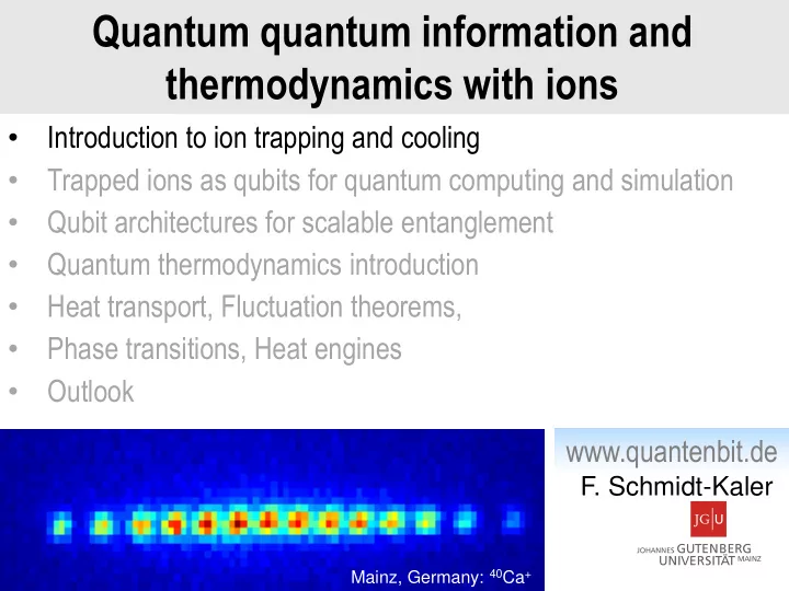
Mainz, Germany: 40Ca+
Quantum quantum information and thermodynamics with ions
SLIDE 2 Ion Gallery
Boulder, USA: Hg+ Aarhus, Denmark: 40Ca+ (red) and 24Mg+ (blue) Oxford, England: 40Ca+ coherent breathing motion of a 7-ion linear crystal Innsbruck, Austria: 40Ca+
SLIDE 3 Why using ions?
- Ions in Paul traps were the first sample with which laser cooling was
demonstrated and quite some Nobel prizes involve laser cooling…
- A single laser cooled ion still represents one of the best understood objects for
fundamental investigations of the interaction between matter and radiation
- Experiments with single ions spurred the development of similar methods with
neutral atoms and solid state physics
- Particular advantages of ions are that they are
- confined to a very small spatial region (dx<l)
- controlled and measured at will for experimental times of days
- strong, long-range coupling
- Ideal test ground for fundamental experiments
- Further applications for
- precision measurements
- quantum computing
- thermodynamics with small systems
- quantum phase transitions
- cavity QED
- optical clocks
- quantum sensors
- exotic matter
SLIDE 4
- Paul trap
- Ion crystals
- Eigenmodes of a linear ion crystal
- Non-harmonic contributions
Introduction to ion trapping
Traditional Paul trap Modern segmented micro Paul trap
SLIDE 5
Dynamic confinement in a Paul trap
SLIDE 6
Invention of the Paul trap
Wolfgang Paul (Nobel prize 1989)
SLIDE 7 Binding in three dimensions
Electrical quadrupole potential Binding force for charge Q leads to a harmonic binding:
no static trapping in 3 dimensions
Laplace equation requires Ion confinement requires a focusing force in 3 dimensions, but such that at least one of the coefficients is negative, e.g. binding in x- and y-direction but anti-binding in z-direction !
trap size:
SLIDE 8 Dynamical trapping: Paul‘s idea
time depending potential with leads to the equation of motion for a particle with charge Q and mass m takes the standard form of the Mathieu equation (linear differential equ. with time depending cofficients) with substitutions radial and axial trap radius
SLIDE 9
Theodor Hänsch‘s video celebrating Wolfgang Paul invention
SLIDE 10 Regions of stability
time-periodic diff. equation leads to Floquet Ansatz If the exponent µ is purely real, the motion is bound, if µ has some imaginary part x is exponantially growing and the motion is unstable. The parameters a and q determine if the motion is stable or not. Find solution analytically (complicated) or numerically: a=0, q =0.1 a=0, q =0.2
time time excursion excursion
a=0, q =0.3 a=0, q =0.4
time time excursion excursion
a=0, q =0.5 a=0, q =0.6
time time excursion excursion
a=0, q =0.7 a=0, q =0.8
time time excursion excursion
a=0, q =0.9 a=0, q =1.0
time time excursion excursion 6 1019
unstable
SLIDE 11 3-Dim. Paul trap stability diagram
for a << q << 1 exist approximate solutions The 3D harmonic motion with frequency wi can be interpreted, approximated, as being caused by a pseudo-potential Y leads to a quantized harmonic oscillator Pseudo potential approximation: RMP 75, 281 (2003), NJP 14, 093023 (2012), PRL 109, 263003 (2012)
SLIDE 12 ideal 3 dim. Paul trap with equi-potental surfaces formed by copper electrodes non-ideal surfaces rring ~ 1.2mm numerical calculation
similar potential near the center
Real 3-Dim. Paul traps
RMP 82, 2609 (2010)
SLIDE 13 x y
2-Dim. Paul mass filter stability diagram
time depending potential with dynamical confinement in the x- y-plane with substitutions radial trap radius
SLIDE 14 Innsbruck design of linear ion trap
1.0mm 5mm
MHz 5
radial
w MHz 2 7 .
axial
w
Blade design
eV depth trap
- F. Schmidt-Kaler, et al.,
- Appl. Phys. B 77, 789 (2003).
SLIDE 15
Ion crystals: Equilibrium positions and eigenmodes
SLIDE 16 Equilibrium positions in the axial potential
z-axis
mutual ion repulsion trap potential find equilibrium positions x0: ions oscillate with q(t) arround condition for equilibrium: dimensionless positions with length scale
B 66, 181 (1998)
SLIDE 17 Equilibrium positions in the axial potential
numerical solution (Mathematica), e.g. N=5 ions equilibrium positions set of N equations for um
0 +0.82 +1.74 force of the trap potential Coulomb force
- f all ions from left side
Coulomb force
- f all ions from left side
SLIDE 18 Eigenmodes and Eigenfrequencies
Lagrangian of the axial ion motion:
m,n=1 m=1 N N
describes small excursions arround equilibrium positions with and
N m,n=1 m=1 N N
B 66, 181 (1998) linearized Coulomb interaction leads to Eigenmodes, but the next term in Tailor expansion leads to mode coupling, which is however typically very small.
- C. Marquet, et al.,
- Appl. Phys. B 76, 199
(2003)
SLIDE 19 Eigenmodes and Eigenfrequencies
Matrix, to diagonize numerical solution (Mathematica), e.g. N=4 ions Eigenvectors Eigenvalues for the radial modes: Market et al., Appl. Phys. B76, (2003) 199
depends on N
pictorial
does not
SLIDE 20 time position
Center of mass mode breathing mode
Common mode excitations
Express / Vol. 3, No. 2 / 89 (1998).
SLIDE 21 Breathing mode excitation
Express / Vol. 3, No. 2 / 89 (1998).
SLIDE 22
- Depends on a=(wax/wrad)2
- Depends on the number of ions acrit= cNb
- Generate a planar Zig-Zag when wax < wy
rad << wx rad
- Tune radial frequencies in y and x direction
1D, 2D, 3D ion crystals
Enzer et al., PRL85, 2466 (2000) Wineland et al., J. Res. Natl. Inst.
- Stand. Technol. 103, 259 (1998)
3D 1D
Kaufmann et al, PRL 109, 263003 (2012)
2D
dx~50nm ±0.25% Planar crystal equilibrium positions
SLIDE 23 Marquet, Schmidt- Kaler, James, Appl.
Ion crystal beyond harmonic approximations
Upot,harm. Ekin UCoulomb
Z0 wavepaket size lz ion distance g,l ion frequencies Dn,m,p coupling matrix
SLIDE 24 Non-linear couplings in ion crystal
Lemmer, Cormick, Schmiegelow, Schmidt-Kaler, Plenio, PRL 114, 073001 (2015)
Self-interaction Cross Kerr coupling Resonant inter-mode coupling
…. remind yourself of non-linear
- ptics: frequency doubling, Kerr
effect, self-phase modulation, ….
SLIDE 25 Resonant inter-mode coupling
two phonons in mode b generate
Non-linear couplings in ion crystal
Cross Kerr coupling
Ding, et al, PRL119, 193602 (2017)
- Frequ. of mode a depends
- n occupation in mode b
SLIDE 26 Basics: Harmonic oscillator
Why? The trap confinement is leads to three independend harmonic oscillators ! here only for the linear direction
- f the linear trap no micro-motion
treat the oscillator quantum mechanically and introduce a+ and a and get Hamiltonian Eigenstates |n> with:
SLIDE 27
Harmonic oscillator wavefunctions
Eigen functions with orthonormal Hermite polynoms and energies:
SLIDE 28 Two – level atom
Why? Is an idealization which is a good approximation to real physical system in many cases
two level system is connected with spin ½ algebra using the Pauli matrices
- D. Leibfried, C. Monroe,
- R. Blatt, D. Wineland,
- Rev. Mod. Phys. 75, 281 (2003)
SLIDE 29 Two – level atom
Why? Is an idealization which is a good approximation to real pyhsical system in many cases
g n , 1 e n , 1 e n, e n , 1 g n , 1 g n,
together with the harmonic oscillator leading to the ladder of eigenstates |g,n>, |e,n>:
levels not coupled
SLIDE 30 2-level-atom harmonic trap
Laser coupling
dressed system
„molecular Franck Condon“ picture
dressed system
g n , 1 e n , 1 e n, e n , 1 g n , 1 g n,
„energy ladder“ picture
SLIDE 31 Laser coupling
dipole interaction, Laser radiation with frequency wl, and intensity |E|2
Rabi frequency:
the laser interaction (running laser wave) has a spatial dependence: Laser
with
momentum kick, recoil:
SLIDE 32 Laser coupling
in the rotating wave approximation
using
and defining the Lamb Dicke parameter h: Raman transition: projection of Dk=k1-k2
x-axis
if the laser direction is at an angle f to the vibration mode direction:
x-axis
single photon transition
SLIDE 33
Lamb Dicke Regime
carrier: red sideband: blue sideband: laser is tuned to the resonances:
SLIDE 34 kicked wave function is non-orthogonal to the other wave functions
Wavefunctions in momentum space
kick by the laser:
SLIDE 35
, g , e 1 , e 1 , g
carrier and sideband Rabi oscillations with Rabi frequencies carrier sideband
Experimental example
and
SLIDE 36
weak confinement: Sidebands are not resolved on that transition. Simultaneous excitation of several vibrational states
„Weak confinement“
g n , 1
e n , 1
e n,
g n,
1, n e +
g n , 1
SLIDE 37 incoherent: W < g
Rabi frequency W W/2p = 5MHz W/2p = 10MHz W/2p = 100MHz W/2p = 50MHz
coherent: W > g
g/2p = 15MHz
Two-level system dynamics
Steady state population of |e>:
Solution of
SLIDE 38 g n , 1 e n , 1 e n, e n , 1 g n , 1 g n,
Rate equations for cooling and heating
cooling:
g n , 1 e n , 1 e n, e n , 1 g n , 1 g n,
heating:
- S. Stenholm, Rev. Mod. Phys. 58, 699 (1986)
probability for population in |g,n>: loss and gain from states with |±n>
loss gain cooling heating
SLIDE 39 Rate equation
different illustration:
n+1 n A- A- A+ A+ g n , 1 e n , 1 e n, e n , 1 g n , 1 g n,
cooling:
g n , 1 e n , 1 e n, e n , 1 g n , 1 g n,
heating:
How to reach red detuning cooling heating steady state phonon number cooling rate
SLIDE 40
weak confinement: Sidebands are not resolved on that transition. Small differences in
„Weak confinement“
detuning for optimum cooling
g n , 1
e n , 1
e n,
g n,
1, n e +
g n , 1
SLIDE 41 weak confinement: Sidebands are not resolved on that transition. Small differences in
„Weak confinement“
detuning for optimum cooling Lorentzian has the steepest slope at
Laser
complications:
- hlaser < hspontaneous
- saturation effects
- optical pumping
- multi-levels
SLIDE 42
g n , 1
e n , 1
g n , 1
g n,
1, n e +
strong confinement – well resolved sidebands: detuning for optimum cooling
g „Strong confinement“
|𝑜, 𝑓 >
SLIDE 43 „Strong confinement“
Laser
strong confinement – well resolved sidebands: detuning for optimum cooling
SLIDE 44
Cooling limit
g ,
e ,
e , 1
g , 1
SLIDE 45 Signature: no further excitation possible „dark state“ |0>
NO!
g ,
e ,
e , 1 g , 2
g , 1
- ptical pumping into the ground state
Sideband ground state cooling
e , 2
SLIDE 46 different methods
- bserve Rabi oscillations on the blue SB
- compare the excitation on the blue SB and the red SB
- compare the excitation on the red SB and the carrier
Experimental: test excitation Pe(t) for D=w and D=w Analysis: Pred/Pblue = m / (m+1)
using:
n=0 n=1
Temperature measurements
SLIDE 47 4.54 4.52 4.5 4.48 0.2 0.4 0.6 0.8 P
D
Detuning dw (MHz) 4.48 4.5 4.52 4.54 0.2 0.4 0.6 0.8 P
D
Detuning dw (MHz) 99.9 % ground state population after sideband cooling after Doppler cooling
7 . 1
z
n
- Ch. Roos et al., Phys. Rev. Lett. 83, 4713 (1999)
Example: ground state cooling
40Ca+
99.9% ground state population
SLIDE 48 P1/2 S1/2 t = 7 ns
397 nm
D5/2
t = 1 s
729 nm
Simplifieds ion energy levels
energy excitation on S1/2 and D5/2
SLIDE 49 P1/2 S1/2 t = 7 ns
397 nm
D5/2
t = 1 s
729 nm Energy Specroscopy pulse followed by detection: Scatter light near 397nm: S1/2 emits fluorescence D5/2 remains dark
„electron shelving
Simplifieds ion energy levels
SLIDE 50 Resolved sideband spectroscopy
Select narrow optical transition with: a) Quadrupole transition b) Raman transition between Hyperfine ground states c) Raman transition between Zeeman ground states d) Octopole transition e) Intercombination line f) RF or MW transitions Species and Isotopes: for (a)
40Ca, 43Ca, 138Ba, 199Hg, 88Sr, ....
for (b)
9Be, 43Ca, 111Cd, 25Mg....
for (c)
40Ca, 24Mg, ....
for (d)
172/172Yb, ....
for (e)
115In, 27Al, ....
for (f)
171Yb, ....
SLIDE 51 Reminder to Doppler cooling
Laser
Problems:
But not into ground state a) Sidebands are not resolved on the transition, small differences in b) Carrier excitation leads to diffusion, heating:
How to shape the atomic resonance line? Quantum-Interference Advantage:
Cools all modes simultaneously Dark resonance: spectrally much sharper than Dopper profile
SLIDE 52 Quantum interference and dark states
L system
S1/2 P1/2 D5/2
Red laser detuning fix blue detuning is scanned
blue detuning [MHz]
D = 0 L system
S1/2 P1/2 D5/2
blue detuning is scanned
blue detuning [MHz]
D = + 55MHz
red laser with detuning fix to the blue side of the resonance
Shape of is no longer Lorentzian
SLIDE 53 Ground state cooling with quantum interference
- G. Morigi, J. Eschner, C. Keitel, Phys. Rev. Lett. 85, 4458 (2000)
transitions are enhanced by bright resonance 1 n n n n transitions are suppressed by quantum interference – no „carrier“ diffusion contribution !
Dr,Wr,kr |e> |r> |g> Dg,Wg,kg
Absorption Detuning Dg
g
2
A b s
p t i
c
i n g l a s e r ( a . u . )
1
1 n n 1 n n 1 n n 1 n n
n n n n
/ ) (
r g
D D
SLIDE 54 Simultaneous ground state cooling of axial and radial motion
axial: P(0)=73% radial: P(0)=58%
lower sidebands upper sidebands
0.1 0.2 0.3 0.4 0.5
S to D excitation probability
1/2 1/2
axial
radial +1.6 MHz radial
axial +3.2 MHz
Simultaneous two mode ground state cooling
Roos et al., Phys. Rev.
SLIDE 55 Simultaneous ground state cooling of 18 axial modes to n~ 0.01..0.02
Multi-mode ground state cooling
Lechner et al, PRA 93, 053401 (2016)
SLIDE 56
- Introduction to ion trapping and cooling
- Trapped ions as qubits for quantum computing and simulation
- Qubit architectures for scalable entanglement
- Quantum thermodynamics introduction
- Heat transport, Fluctuation theorems,
- Phase transitions, Heat engines
- Outlook
www.quantenbit.de
Mainz, Germany: 40Ca+
Quantum quantum information and thermodynamics with ions