posterior distributions
play

Posterior distributions p ( |D , M ) = P ( D| ) p ( ) P ( D|M ) - PowerPoint PPT Presentation

Deterministic Approximations 2 Posterior distributions p ( |D , M ) = P ( D| ) p ( ) P ( D|M ) Laplace and variational approximations E.g., logistic regression: p ( ) = N ( ; 0 , 2 I ) labels z ( n ) 1 ( z ( n ) w


  1. Deterministic Approximations 2 Posterior distributions p ( θ |D , M ) = P ( D| θ ) p ( θ ) P ( D|M ) Laplace and variational approximations E.g., logistic regression: p ( θ ) = N ( θ ; 0 , σ 2 I ) � labels z ( n ) ∈ ± 1 σ ( z ( n ) w ⊤ x ( n ) ) , P ( D| θ ) = Integrate large product non-linear functions. Goals: summarize posterior in simple form, Iain Murray estimate model evidence P ( D|M ) http://iainmurray.net/ 
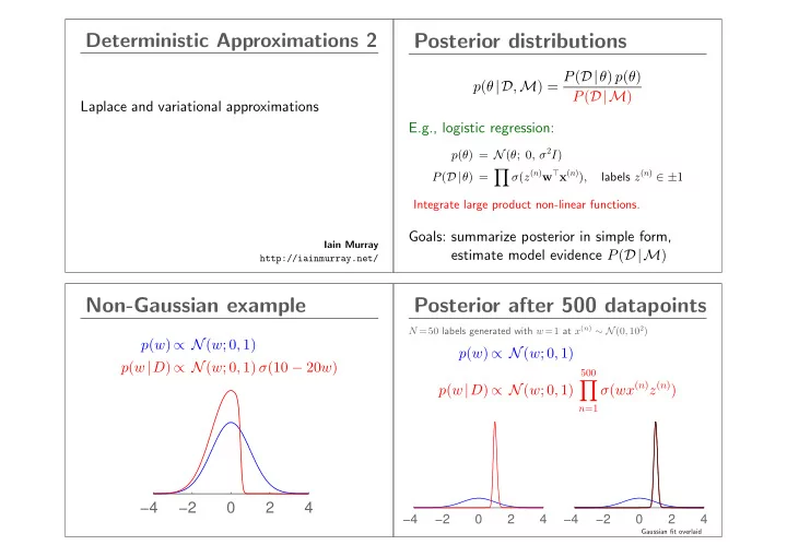
Non-Gaussian example Posterior after 500 datapoints N =50 labels generated with w =1 at x ( n ) ∼ N (0 , 10 2 ) p ( w ) ∝ N ( w ; 0 , 1) p ( w ) ∝ N ( w ; 0 , 1) p ( w | D ) ∝ N ( w ; 0 , 1) σ (10 − 20 w ) 500 � σ ( wx ( n ) z ( n ) ) p ( w | D ) ∝ N ( w ; 0 , 1) n =1 −4 −2 0 2 4 −4 −2 0 2 4 −4 −2 0 2 4 Gaussian fit overlaid

  2. Gaussian approximations Laplace Approximation MAP estimate: Finite parameter vector θ θ ∗ = arg max � � log P ( D| θ ) + log P ( θ ) . θ P ( θ | lots of data ) often nearly Gaussian around the mode Taylor expand at optimum: − log P ( θ |D ) = E ( θ ) = − log P ( D| θ ) − log P ( θ ) + log P ( D ) . Need to identify which Gaussian it is: mean, covariance Because ∇ θ E is zero at θ ∗ (a turning point): E ( θ ∗ + δ ) ≃ E ( θ ∗ ) + 1 2 δ ⊤ H δ Do same thing to Gaussian around mean, identify Laplace approximation: P ( θ |D ) ≈ N ( θ ; θ ∗ , H − 1 ) Laplace details Laplace picture Matrix of second derivatives is called the Hessian: �� ∂ 2 � � H ij = − log P ( θ |D ) � ∂θ i ∂θ j � θ = θ ∗ Find posterior mode (MAP estimate) θ ∗ using favourite gradient-based optimizer. Curvature and mode match. Log posterior doesn’t need to be normalized: constants We can normalize Gaussian. Height at mode won’t match exactly! disappear from derivatives and second-derivatives Used to approximate model likelihood (AKA ‘evidence’, ‘marginal likelihood’): ≈ P ( D| θ ∗ ) P ( θ ∗ ) P ( D ) = P ( D| θ ) P ( θ ) 1 N ( θ ∗ ; θ ∗ , H − 1 ) = P ( D| θ ∗ ) P ( θ ∗ ) | 2 πH − 1 | 2 P ( θ |D )

  3. Laplace problems Other Gaussian approximations Can match a Gaussian in other ways that derivatives Weird densities (we’ve seen sometimes happen) won’t work well. We only locally match one mode. Accurate approximation with Gaussian may not be possible Mode may not have much mass, or misleading curvature High dimensions: mode may be flat in some direction Capturing posterior width better than only fitting point estimate → ill-conditioned Hessian Variational methods Kullback–Leibler Divergence � p ( θ ) log p ( θ ) D KL ( p || q ) = q ( θ ) d θ Goal: fit target distribution (e.g., parameter posterior) Define: D KL ( p || q ) ≥ 0 . Minimized by p ( θ ) = q ( θ ) . — family of possible distributions q ( θ ) — ‘variational objective’ (says ‘how well does q match?’) Information theory (non-examinable for MLPR): KL divergence: average storage wasted by Optimize objective: compression system using model q instead of Fit parameters of q ( θ ) — e.g., mean and cov of Gaussian true distribution p .

  4. Minimizing D KL ( p || q ) Minimizing D KL ( p || q ) Select family: q ( θ ) = N ( θ ; µ, Σ) , Optimizing D KL ( p || q ) tends to be hard. Minimize D KL ( p || q ) : match mean and cov of p . Even Gaussian q : mean and cov of p ? MCMC? Answer may not be what you want: −4 −2 0 2 4 Considering D KL ( q || p ) D KL ( q || p ) : fitting posterior Fit q to p ( θ |D ) = p ( D| θ ) p ( θ ) p ( D ) Substitute into KL and get spray of terms: D KL ( q || p ) = E q [log q ( θ )] − E q [log p ( D| θ )] min KL ( p || q ) local min KL ( q || p ) local min KL ( q || p ) − E q [log p ( θ )] + log p ( D ) � � D KL ( q || p ) = − q ( θ ) log p ( θ |D ) d θ + q ( θ ) log q ( θ ) d θ First three terms: Minimize sum of these, J ( q ) . � �� � log p ( D ) : Model evidence. Usually intractable, but: neg. entropy, − H ( q ) D KL ( q || p ) ≥ 0 ⇒ log p ( D ) ≥ − J ( q ) 1. “Don’t put probability mass on implausible parameters” 2. Want to be spread out, high entropy. We optimize lower bound on the log marginal likelihood

  5. D KL ( q || p ) : optimization Summary Laplace approximation: Literature full of clever (non-examinable) iterative ways to — Straightforward to apply; accuracy variable optimize D KL ( q || p ) . q not always Gaussian. — 2nd derivatives → certainty of parameter Use standard optimizers? Hardest term to evaluate is: — Incremental improvement on MAP estimate N � E q [log p ( D| θ )] = E q [log p ( x n | θ )] Variational methods: n =1 — Fit variational parameters of q (not θ !) Sum of possibly simple integrals. — KL ( p || q ) vs. KL ( q || p ) Stochastic gradient descent is an option. — Bound marginal/model likelihood (‘the evidence’)

Download Presentation
Download Policy: The content available on the website is offered to you 'AS IS' for your personal information and use only. It cannot be commercialized, licensed, or distributed on other websites without prior consent from the author. To download a presentation, simply click this link. If you encounter any difficulties during the download process, it's possible that the publisher has removed the file from their server.

Recommend


More recommend