Perfect competition with real firms 1 Topic 3 Topic 4 Topic 5 - - PDF document

P1 Sep–Oct 2012 • Timothy Van Zandt • Prices & Markets Session 6 • Applications of Perfect Competition Page 1

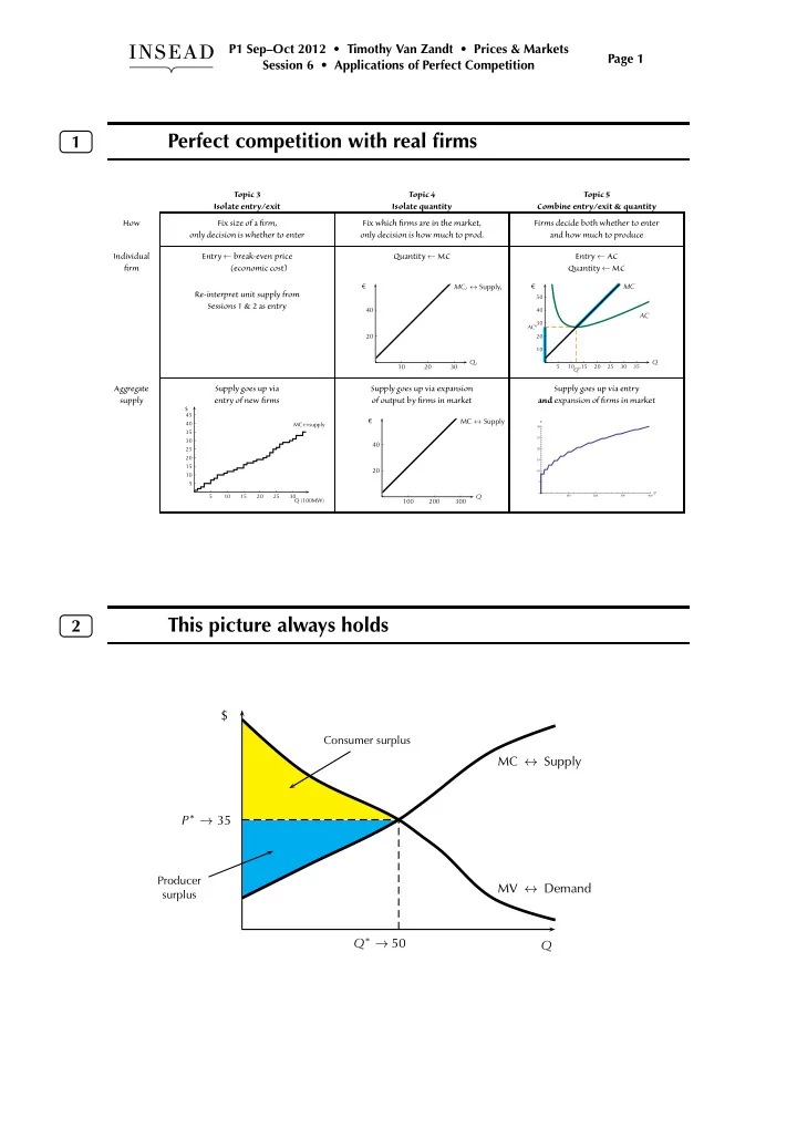
1

Perfect competition with real firms

Topic 3 Topic 4 Topic 5 Isolate entry/exit Isolate quantity Combine entry/exit & quantity How Fix size of a firm, Fix which firms are in the market, Firms decide both whether to enter

• nly decision is whether to enter
• nly decision is how much to prod.

and how much to produce Individual Entry ← break-even price Quantity ← MC Entry ← AC firm (economic cost) Quantity ← MC Re-interpret unit supply from Sessions 1 & 2 as entry

20 40 10 20 30

MCi ↔ Supplyi €

Qi

10 20 30 40 50 5 10 15 20 25 30 35

AC MC €

Q

Qu ACu

Aggregate Supply goes up via Supply goes up via expansion Supply goes up via entry supply entry of new firms

• f output by firms in market

and expansion of firms in market

MC↔supply 5 10 15 20 25 30 35 40 45 5 10 15 20 25 30 Q (100MW) $

20 40 100 200 300

MC ↔ Supply €

Q

100 200 300 400 Q 5 10 15 20 25 30 P

2

This picture always holds

$ Q

Producer surplus Consumer surplus

P∗ → 35 Q∗ → 50 MV ↔ Demand MC ↔ Supply

P1 Sep–Oct 2012 • Timothy Van Zandt • Prices & Markets Session 6 • Applications of Perfect Competition Page 2

3

• 6. Applications of Perfect Competition

1. ➥ Market dynamics.

• 2. Simulation results.
• 3. Bagels and Cranberries (“Growth and Profitability”).

4

Long-run dynamics

$ Q

10 20 30 40 50 60 10 20 30 40 50 60 70 80 90 P∗

1 →

P∗

2 →

D1 D2 Slong

P1 Sep–Oct 2012 • Timothy Van Zandt • Prices & Markets Session 6 • Applications of Perfect Competition Page 3

5

Firms’ short-run responses to price changes

$ Q

10 20 30 40 50 60 10 20 30 40 50 60 70 80 90 P∗

1 →

D1 Slong

6

Short-run vs. long-run price adjustment

$ Q

10 20 30 40 50 60 10 20 30 40 50 60 70 80 90

D1 D2 Slong Sshort

P1 Sep–Oct 2012 • Timothy Van Zandt • Prices & Markets Session 6 • Applications of Perfect Competition Page 4

7

Bottom line

Whatever the source of adjustment delays and costs: Adjustment delays and costs imply that supply adjusts less in the short run than in the long run—hence, prices are more volatile in the short run than in the long run.

8

Interpreted as delays for entry

$ Q

10 20 30 40 50 60 10 20 30 40 50 60 70 80 90

D1 D2 Slong Sshort

P1 Sep–Oct 2012 • Timothy Van Zandt • Prices & Markets Session 6 • Applications of Perfect Competition Page 5

9

Price and capacity dynamics in a competitive industry

• (Courtesy of David Besanko.)

10

Bulk shipping

Bulk shipping: vessels designed to carry a homogeneous unpacked dry or liquid cargo, for individual shippers on non-scheduled routes.

• Common cargo: iron ore, grain, coal, bauxite, phosphates, steel,

cement, sugar, wood chips.

• “Taxis, not buses”. (Entire cargo belongs to one shipper.)
• 72% of world seaborn trade (by weight).

(Data is thanks to Myrto Kaloupsidi.)

P1 Sep–Oct 2012 • Timothy Van Zandt • Prices & Markets Session 6 • Applications of Perfect Competition Page 6

11

Market structure

12

Shipping prices

P1 Sep–Oct 2012 • Timothy Van Zandt • Prices & Markets Session 6 • Applications of Perfect Competition Page 7

13

Demand volatility

Maarket is characterized by demand volatility due to changing export patterns, macroeconomic cycles.

14

Elasticity

• 1. Transportation costs are a small portion of total cost for most goods

(e.g. for gasoline $0.07 per gallon).

• 2. Few short-run substitutes.
• 3. Disruptions are costly:
• “Just-in-time” inventory models
• “Continuous-flow” refining

So what?

P1 Sep–Oct 2012 • Timothy Van Zandt • Prices & Markets Session 6 • Applications of Perfect Competition Page 8

15

Demand volatility

Demand: inelastic and volatile + Supply: inelastic ⇓

Volatile prices

16

• 6. Applications of Perfect Competition

1. ✓ Market dynamics. 2. ➥ Simulation results.

• 3. Bagels and Cranberries (“Growth and Profitability”).

P1 Sep–Oct 2012 • Timothy Van Zandt • Prices & Markets Session 6 • Applications of Perfect Competition Page 9

17

• 6. Applications of Perfect Competition

1. ✓ Market dynamics. 2. ✓ Simulation results. 3. ➥ Bagels and Cranberries (“Growth and Profitability”).

18

• 6. Applications of Perfect Competition

1. ✓ Market dynamics. 2. ✓ Simulation results. 3. ✓ Bagels and Cranberries (“Growth and Profitability”).

P1 Sep–Oct 2012 • Timothy Van Zandt • Prices & Markets Session 6 • Applications of Perfect Competition Page 10

19

This week

(Wed) Session 7: Elasticity of demand

• Prep Guide 8.
• FPM Ch. 8.
• A demand estimation exercise to hand in.

(Fri) Session 8: Pricing with Market Power

• Prep Guide 7.
• FPM Ch. 7.

20

Reminder: Next week you have …

… optional review and quiz.

Monday Tuesday Wednesday Thursday Friday Session 9 Review Quiz Session 10 –

Quiz covers only up through Session 8.

One way to approach your task in rounds 1 and 2:

• 1. Predict a market price P .
• 2. Decide how much to produce at this price: si(P) .
• 3. Back out inputs needed to produce this amount.

Supply curve? Derive from cost curve. Cost curve? Derive from production function.

Total cost:

5000 10000 100 200 300

€ Q c(Q)

Individual firm: Production function:

f (L, M) = L1/3M1/3

⇓

Derive cost curve:

c(Q) = 2Q3/2

⇓

Marginal cost:

mc(Q) = 3Q1/2

⇓

Inverse is supply curve:

si(P) = P2/9

Marginal cost / Supply:

30 60 90 100 200 300

€ Q mc(Q) , si(P)

Higher level question – how to predict P ?

Forecasts Individual supply Aggregate supply Market price

Equilibrium: s(P) = d(P) . Equilibrium: Total supply:

39 × si(P)

⇒

s(P) = 39 9 P2

• Equil. solves:

s(P) = d(P)

⇒

P∗ = 27.42

Back to you: You choose:

Qi = si(P∗)

⇒

Qi = 83.5

Back out inputs: from f

⇒

L = M = 763.5

Supply / Demand / Equilibrium:

30 60 90 3000 6000 9000

€ Q d(P) s(P)

Following the shift in demand … Short-run problem (Round 3): Machines are fixed at their round-2 level. Long-run problem (Rounds 4, 5): Both inputs are adjustable. Long-run adjustment: New demand:

dnew(P) = 8970 − 100P

Equilibrium:

s(P) = dnew(P)

⇒

Pnew = 35.40

Back to you: You choose:

Qi = si(Pnew)

⇒

Qi = 5430

Back out inputs: from f

⇒

L4 = M4 = 1643

New Long-run Equilibrium:

30 60 90 3000 6000 9000

€ Q d(P) s(P) New long-run equilibrium dnew(P)

Short-run production (round 3): Stuck with:

Mcurr = 763.5

Short-run prod. function

Q = L1/3M1/3

curr

invert

⇓

Labor requirements:

L = Q3 Mcurr

Total cost:

5000 10000 100 200 300

€ Q c(Q)

• c(Q)

Short-run costs (round 3):

( = short-run values)

Total cost:

• c(Q) = Mcurr + Q3

Mcurr

short-run fixed cost short-run variable cost

Marginal cost:

• mc(Q) =

3 Mcurr Q2

(Invert P = MC)

⇓

Supply:

• si(Q) =
• Mcurr

3 P

Marginal cost / Supply:

30 60 90 100 200 300

€ Q mc(Q) , si(P)

• mcs(Q) ,

si(P)

Short-run equilibrium (round 3): Total supply:

ˆ

s(P) = 39 × si(P)

Equilibrium:

• s(P) = dnew(P)

⇒

• P = 47.03

Back to you: You choose:

• Qi =

si( P)

⇒

• Qi = 109.4

Back out inputs: from f

⇒

L3 = 1715

Short-run equilibrium:

30 60 90 3000 6000 9000

€ Q d(P)

• s(P)

Short-run equilibrium dnew(P)

Short-run and Long-run Equilibria:

30 60 90 3000 6000 9000

€ Q d(P) s(P)

• s(P)

dnew(P)

Short-run and Long-run Equilibria:

Round

P Qi Li Mi

1, 2 27.42 83.5 763.5 763.5 3 47.03 109.4 1715 4, 5 35.40 139.2 1643 1643

Short-run and Long-run Equilibria:

90 3000 6000 9000

60 € Q d(P) s(P) dnew(P)

• s(P)

27.42 35.40 47.03

What Actually Happened:

Round

P Qi

1 29.82 77 2 28.41 81 3 47.59 108 4 37.42 134 5 34.18 142

What Actually Happened:

90 3000 6000 9000

60 € Q d(P) s(P) dnew(P)

• s(P)

R1 R2 R3 R4 R5