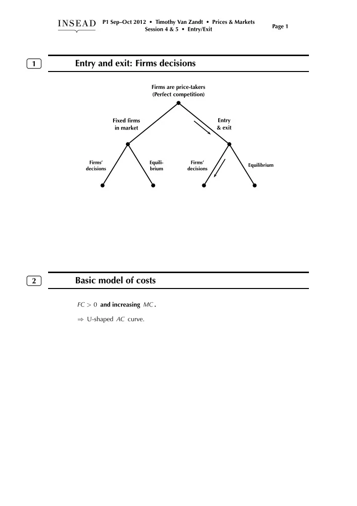
[PDF] - Entry and exit: Firms decisions 1 Firms are price-takers (Perfect PDF Document

SLIDE 1

P1 Sep–Oct 2012 • Timothy Van Zandt • Prices & Markets Session 4 & 5 • Entry/Exit Page 1

1 Entry and exit: Firms decisions

Firms are price-takers (Perfect competition) Fixed firms in market

Firms’ decisions Equili- brium

Entry & exit

Firms’ decisions Equilibrium

2 Basic model of costs

FC > 0 and increasing MC . ⇒ U-shaped AC curve.

SLIDE 2

P1 Sep–Oct 2012 • Timothy Van Zandt • Prices & Markets Session 4 & 5 • Entry/Exit Page 2

3 Quantity decision depends only on the MC curve

1 2 3 4 5 6 7 8 10 20 30 40 50 60 70

€

Q

MC

4 Entry decision depends only the AC curve

1 2 3 4 5 6 7 8 10 20 30 40 50 60 70

€

Q

AC

SLIDE 3

P1 Sep–Oct 2012 • Timothy Van Zandt • Prices & Markets Session 4 & 5 • Entry/Exit Page 3

5 Can combine to see entry and scale decisions at same time

1 2 3 4 5 6 7 8 10 20 30 40 50 60 70

€

Q

AC MC

6 Exercise 3.8

TC = 144 + 3Q + Q2 FC = 144 constant/intercept MC = 3 + 2Q derivative AC = 144 Q + 3 + Q TC/Q Qu = 12 solves MC = AC ACu = 27 = ac(Qu) = mc(Qu)

SLIDE 4

P1 Sep–Oct 2012 • Timothy Van Zandt • Prices & Markets Session 4 & 5 • Entry/Exit Page 4

7 MC curve

10 20 30 40 50 5 10 15 20 25 30 35

8 AC curve

10 20 30 40 50 5 10 15 20 25 30 35

SLIDE 5

P1 Sep–Oct 2012 • Timothy Van Zandt • Prices & Markets Session 4 & 5 • Entry/Exit Page 5

9 Together

10 20 30 40 50 5 10 15 20 25 30 35

AC MC €

Q

Qu ACu

10 Exercise 4.5: What if MC goes up by 10

10 20 30 40 50 5 10 15 20 25 30 35

AC MC €

Q

Qu ACu

SLIDE 6

P1 Sep–Oct 2012 • Timothy Van Zandt • Prices & Markets Session 4 & 5 • Entry/Exit Page 6

11 Exercise 4.6: What if FC goes up?

10 20 30 40 50 5 10 15 20 25 30 35

AC MC €

Q

Qu ACu

12 Entry and exit: equilibrium

Firms are price-takers (Perfect competition) Fixed firms in market

Firms’ decisions Equili- brium

Entry & exit

Firms’ decisions Equilibrium

SLIDE 7

P1 Sep–Oct 2012 • Timothy Van Zandt • Prices & Markets Session 4 & 5 • Entry/Exit Page 7

13 Aggregate supply and equilibrium?

14 A two-stage view

(Entry, then competition between firms in the market.)

A B C D E F G H I J K

M a r k e t

SLIDE 8

P1 Sep–Oct 2012 • Timothy Van Zandt • Prices & Markets Session 4 & 5 • Entry/Exit Page 8

15 How would you calculate a numerical example?

Simplification: Firms have same MC – heterogeneity is through the FC Then equilibrium depends on # of firms, not their identities

16 Here is such an example

Data (cost curve, demand curve) are from simulation rounds 1&2

N P Qi Vi Equilibrium as function of N

1 56.46 354 6,665 2 53.61 319 5,707 3 51.25 292 4,984 4 49.23 269 4,419 5 47.48 250 3,964 6 45.93 234 3,590 7 44.56 221 3,277 8 43.32 209 3,011 9 42.20 198 2,782 10 41.17 188 2,584 11 40.22 180 2,410 12 39.35 172 2,257 13 38.54 165 2,121 14 37.79 159 1,998 15 37.08 153 1,889 16 36.42 147 1,789 17 35.80 142 1,699 18 35.21 138 1,616 19 34.65 133 1,541 20 34.12 129 1,472 21 33.62 126 1,408 22 33.15 122 1,349 23 32.69 119 1,294 24 32.26 116 1,243 25 31.84 113 1,195

SLIDE 9

P1 Sep–Oct 2012 • Timothy Van Zandt • Prices & Markets Session 4 & 5 • Entry/Exit Page 9

17 Now consider pool of potential firms

FC ACu Potential Entrants

50 11.05 150 15.94 250 18.90 350 21.14 450 22.99 550 24.58 650 25.99 750 27.26 850 28.42 950 29.49 1,050 30.49 1,150 31.43 1,250 32.32 1,350 33.16 1,450 33.96 1,550 34.72 1,650 35.45 1,750 36.15 1,850 36.83 1,950 37.48 2,050 38.11 2,150 38.72 2,250 39.31 2,350 39.89 2,450 40.44

18 Put the data together

N P Qi Vi Equilibrium as function of N

1 56.46 354 6,665 2 53.61 319 5,707 3 51.25 292 4,984 4 49.23 269 4,419 5 47.48 250 3,964 6 45.93 234 3,590 7 44.56 221 3,277 8 43.32 209 3,011 9 42.20 198 2,782 10 41.17 188 2,584 11 40.22 180 2,410 12 39.35 172 2,257 13 38.54 165 2,121 14 37.79 159 1,998 15 37.08 153 1,889 16 36.42 147 1,789 17 35.80 142 1,699 18 35.21 138 1,616 19 34.65 133 1,541 20 34.12 129 1,472 21 33.62 126 1,408 22 33.15 122 1,349 23 32.69 119 1,294 24 32.26 116 1,243 25 31.84 113 1,195

FC ACu Potential Entrants

50 11.05 150 15.94 250 18.90 350 21.14 450 22.99 550 24.58 650 25.99 750 27.26 850 28.42 950 29.49 1,050 30.49 1,150 31.43 1,250 32.32 1,350 33.16 1,450 33.96 1,550 34.72 1,650 35.45 1,750 36.15 1,850 36.83 1,950 37.48 2,050 38.11 2,150 38.72 2,250 39.31 2,350 39.89 2,450 40.44

SLIDE 10

P1 Sep–Oct 2012 • Timothy Van Zandt • Prices & Markets Session 4 & 5 • Entry/Exit Page 10

19 Identical firms (free entry)

Recipe:

1. P∗ =
2. Q∗

i =

3. Q∗ =
4. N∗ =

20 Example

Each firm: TC = 144 + 3Q + Q2 FC = 144 MC = 3 + 2Q AC = 144 Q + 3 + Q Qu = 12 ACu = 27

20 40 10 20 30

AC MC €

Q

Qu ACu

Demand: Q = 510 − 10P

1. P∗ =
2. Q∗

i =

3. Q∗ =
4. N∗ =

SLIDE 11

P1 Sep–Oct 2012 • Timothy Van Zandt • Prices & Markets Session 4 & 5 • Entry/Exit Page 11

21 Exercise 5.5: What if MC goes up by 10?

(a) Q∗

i

(b) P∗ (c) Q∗ (d) N∗

22 Exercise 5.6: What if the FC goes up?

(a) Q∗

i

(b) P∗ (c) Q∗ (d) N∗

SLIDE 12

P1 Sep–Oct 2012 • Timothy Van Zandt • Prices & Markets Session 4 & 5 • Entry/Exit Page 12

23 Numerical example to illustrate 5.6

N P Qi Vi Equilibrium as function of N

1 56.46 354 6,665 2 53.61 319 5,707 3 51.25 292 4,984 4 49.23 269 4,419 5 47.48 250 3,964 6 45.93 234 3,590 7 44.56 221 3,277 8 43.32 209 3,011 9 42.20 198 2,782 10 41.17 188 2,584 11 40.22 180 2,410 12 39.35 172 2,257 13 38.54 165 2,121 14 37.79 159 1,998 15 37.08 153 1,889 16 36.42 147 1,789 17 35.80 142 1,699 18 35.21 138 1,616 19 34.65 133 1,541 20 34.12 129 1,472 21 33.62 126 1,408 22 33.15 122 1,349 23 32.69 119 1,294 24 32.26 116 1,243 25 31.84 113 1,195

FC 900 1300 ACu 38.97 42.80 N∗

22 15

P∗

39.05 42.86

Q∗

i

95 114

24 And if the demand curve shifted to the right?

1 2 3 4 5 6 7 8 9 1 1 1 1 1 1 1 1 1 1 2 2 2 2 2 2 2 2

N P Qi V∏i Equilibrium as function of N

1 56.46 354 6,665 2 53.61 319 5,707 3 51.25 292 4,984 4 49.23 269 4,419 5 47.48 250 3,964 6 45.93 234 3,590 7 44.56 221 3,277 8 43.32 209 3,011 9 42.20 198 2,782 10 41.17 188 2,584 11 40.22 180 2,410 12 39.35 172 2,257 13 38.54 165 2,121 14 37.79 159 1,998 15 37.08 153 1,889 16 36.42 147 1,789 17 35.80 142 1,699 18 35.21 138 1,616 19 34.65 133 1,541 20 34.12 129 1,472 21 33.62 126 1,408 22 33.15 122 1,349 23 32.69 119 1,294 24 32.26 116 1,243 25 31.84 113 1,195 26 31.44 110 1,151 27 31.06 107 1,110

FC ACu Potential Entrants

50 11.05 150 15.94 250 18.90 350 21.14 450 22.99 550 24.58 650 25.99 750 27.26 850 28.42 950 29.49 1,050 30.49 1,150 31.43 1,250 32.32 1,350 33.16 1,450 33.96 1,550 34.72 1,650 35.45 1,750 36.15 1,850 36.83 1,950 37.48 2,050 38.11 2,150 38.72 2,250 39.31 2,350 39.89 2,450 40.44 2,550 40.99 2,650 41.51 1 2 3 4 5 6 7 8 9 1 1 1 1 1 1 1 1 1 1 2 2 2 2 2 2 2 2

N P Qi V∏i Equilibrium as function of N

1 82.19 751 20,566 2 76.65 653 16,676 3 72.28 581 13,988 4 68.71 525 12,017 5 65.71 480 10,509 6 63.13 443 9,319 7 60.88 412 8,356 8 58.88 385 7,561 9 57.10 362 6,894 10 55.49 342 6,328 11 54.03 324 5,840 12 52.69 308 5,417 13 51.46 294 5,046 14 50.32 281 4,718 15 49.26 270 4,427 16 48.27 259 4,166 17 47.35 249 3,932 18 46.48 240 3,720 19 45.67 232 3,528 20 44.90 224 3,353 21 44.17 217 3,192 22 43.48 210 3,045 23 42.83 204 2,909 24 42.20 198 2,784 25 41.61 192 2,668 26 41.04 187 2,560 27 40.50 182 2,460