
SLIDE 1
P1 Sep–Oct 2012 • Timothy Van Zandt • Prices & Markets Review Session Page 1
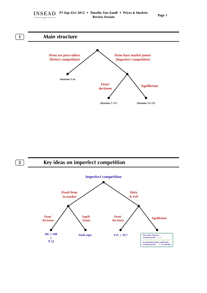
1
Main structure
(Sessions 1–6)
(Firms’ decisions & equilibrium)
Firms are price-takers (Perfect competition) Firms have market power (Imperfect competition)
(Sessions 7–11)
Firms’ decisions
(Sessions 12–15)
Equilibrium
In each case: fixed firms in the market, then entry/exit
2
Key ideas on imperfect competition
Imperfect competition
Fixed firms in market
MC = MR ⇓ P, Q Firms’ decisions Nash eqm. Equili- brium
Entry & exit
VΠ > FC? Firms’ decisions
Each active firm has economic profit ≥ 0 . No potential entrant could make economic profit > 0 by entering.