4 Game Trees Game tree 4 Game Trees Game tree perfect information - PDF document

§4 Game Trees Game tree §4 Game Trees Game tree � perfect information games perfect information games � all possible plays of two all possible plays of two- -player, perfect player, perfect � � � no hidden information no hidden information information games can be represented with a � information games can be represented with a � two two- -player, perfect information games player, perfect information games � game tree game tree � Noughts and Crosses Noughts and Crosses � � nodes: positions (or states) nodes: positions (or states) � Chess Chess � � � Go Go � � edges: moves edges: moves � � imperfect information games imperfect information games � � players: players: MAX MAX (has the first move) and (has the first move) and MIN � MIN � Poker Poker � � Backgammon Backgammon � ply = the length of the path between two nodes ply = the length of the path between two nodes � � � Monopoly Monopoly � MAX has even plies counting from the root node has even plies counting from the root node � MAX � zero zero- -sum property sum property � � MIN has odd plies counting from the root node has odd plies counting from the root node � one player’s gain equals another player’s loss one player’s gain equals another player’s loss � MIN � � 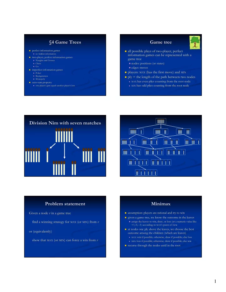Division Nim with seven matches Division Nim with seven matches Problem statement Problem statement Minimax Minimax Given a node v Given a node v in a game tree in a game tree � assumption: players are rational and try to win assumption: players are rational and try to win � � given a game tree, we know the outcome in the leaves given a game tree, we know the outcome in the leaves � find a winning strategy for find a winning strategy for MAX MAX (or (or MIN MIN ) from ) from v v � assign the leaves to win, draw, or loss (or a numeric value like assign the leaves to win, draw, or loss (or a numeric value like � +1, 0, – –1) according to 1) according to MAX ’s point of view +1, 0, MAX ’s point of view � at nodes one ply above the leaves, we choose the best at nodes one ply above the leaves, we choose the best � or (equivalently) or (equivalently) outcome among the children (which are leaves) outcome among the children (which are leaves) MAX : win if possible; otherwise, draw if possible; else loss : win if possible; otherwise, draw if possible; else loss � MAX � show that MAX MAX (or (or MIN ) can force a win from v v show that MIN ) can force a win from : loss if possible; otherwise, draw if possible; else win MIN : loss if possible; otherwise, draw if possible; else win � MIN � � recurse through the nodes until in the root recurse through the nodes until in the root � 1

MAX MAX –1 Minimax rules Minimax rules MIN MIN –1 –1 –1 If the node is labelled to MAX If the node is labelled to MAX , assign it to the , assign it to the 1. 1. maximum value of its children. maximum value of its children. MAX MAX If the node is labelled to MIN , assign it to the If the node is labelled to MIN , assign it to the +1 –1 +1 –1 2. 2. minimum value of its children. minimum value of its children. MIN MIN +1 –1 +1 MIN minimizes, minimizes, MAX MAX maximizes → minimax maximizes → minimax MIN � � MAX MAX +1 –1 MIN MIN +1 Rough estimates on running Rough estimates on running Analysis Analysis times when d times when d = 5 = 5 � simplifying assumptions simplifying assumptions � suppose expanding a node takes 1 ms suppose expanding a node takes 1 ms � � � internal nodes have the same branching factor internal nodes have the same branching factor b b � � branching factor branching factor b b depends on the game depends on the game � � game tree is searched to a fixed depth game tree is searched to a fixed depth d d � � Draughts ( Draughts ( b b ≈ 3): ≈ 3): t t = 0.243 s = 0.243 s � time consumption is proportional to the number of time consumption is proportional to the number of � � expanded nodes expanded nodes � Chess ( Chess ( b b ≈ 30): ≈ 30): t t = 6 = 6¾ ¾ h h � � 1 1 — — root node (the initial ply) root node (the initial ply) � � Go ( Go ( b b ≈ 300): ≈ 300): t t = 77 a = 77 a � � b b — — nodes in the first ply nodes in the first ply � 2 — � b b 2 — nodes in the second ply nodes in the second ply � alpha alpha- -beta pruning reduces beta pruning reduces b b � � d — � b b d — nodes in the nodes in the d d th ply th ply � � overall running time overall running time O O ( ( b b d d ) ) � Controlling the search depth Controlling the search depth Evaluation function Evaluation function � usually the whole game tree is too large usually the whole game tree is too large � combination of numerical measurements combination of numerical measurements � � → limit the search depth → limit the search depth m m i i ( ( s s , , p p ) of the game state ) of the game state → a partial game tree → a partial game tree � single measurement: single measurement: m m i i ( ( s s , , p p ) ) � → partial minimax → partial minimax � difference measurement: difference measurement: m m i i ( ( s s , , p p ) − ) − m m j j ( ( s s , , q q ) ) � � n n - -move look move look- -ahead strategy ahead strategy � ratio of measurements: ratio of measurements: m m i i ( ( s s , , p p ) / ) / m m j j ( ( s s , , q q ) ) � � � stop searching after stop searching after n n moves moves � aggregate the measurements maintaining the aggregate the measurements maintaining the � � zero- -sum property sum property � make the internal nodes (i.e., frontier nodes) leaves make the internal nodes (i.e., frontier nodes) leaves zero � � use an evaluation function to ‘guess’ the outcome use an evaluation function to ‘guess’ the outcome � 2

Example: Noughts and Crosses Examples of the evaluation Example: Noughts and Crosses Examples of the evaluation � heuristic evaluation function heuristic evaluation function e e : : � e e (•) = (•) = 6 6 – – 5 5 = 1 = 1 � count the winning lines open to count the winning lines open to MAX � MAX � subtract the number of winning lines open to subtract the number of winning lines open to MIN � MIN � forced wins forced wins � � state is evaluated + ∞ , if it is a forced win for state is evaluated + ∞ , if it is a forced win for MAX � MAX e e (•) = (•) = 4 4 – – 5 5 = = – –1 1 � state is evaluated state is evaluated – – ∞ , if it is forced win for ∞ , if it is forced win for MIN � MIN e (•) = + ∞ (•) = + ∞ e The deeper the better...? Drawbacks of partial minimax The deeper the better...? Drawbacks of partial minimax � assumptions: assumptions: � horizon effect horizon effect � � � n n - -move look move look- -ahead ahead � heuristically promising path can lead to an unfavourable heuristically promising path can lead to an unfavourable � � � branching factor branching factor b b , depth , depth d d , , situation situation � � leaves with uniform random distribution leaves with uniform random distribution � staged search: extend the search on promising nodes staged search: extend the search on promising nodes � � � minimax convergence theorem: minimax convergence theorem: � � iterative deepening: increase iterative deepening: increase n n until out of memory or time until out of memory or time � � n n increases → root value converges to increases → root value converges to f f ( ( b b , , d d ) ) � phase phase- -related search: opening, midgame, end game related search: opening, midgame, end game � � � last player theorem: last player theorem: � � however, horizon effect cannot be totally eliminated however, horizon effect cannot be totally eliminated � � root values from odd and even plies not comparable root values from odd and even plies not comparable � � bias bias � � minimax pathology theorem: minimax pathology theorem: � � we want to have an estimate of minimax but get a minimax of we want to have an estimate of minimax but get a minimax of � � n n increases → probability of selecting non increases → probability of selecting non- -optimal move optimal move estimates estimates � increases ( ← uniformity assumption!) increases ( ← uniformity assumption!) � distortion in the root: odd plies → win, even plies → loss distortion in the root: odd plies → win, even plies → loss � 3