Overview Recursive Ray Tracing Shadow Feelers Snells Law for - - PDF document

Ray-tracing Overview

 Recursive Ray Tracing  Shadow Feelers  Snell’s Law for Refraction  When to stop!

Recap: Light Transport

Recap: Local Illumination

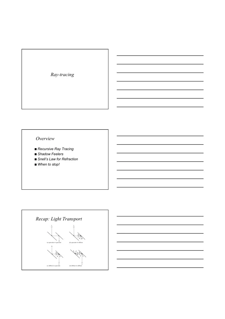
 Ambient, diffuse & specular components  The sum is over the specular and diffuse

components for each light

( ) ( )

( )

∑ =

⋅ + ⋅ + =

M j m j s j d j i a r

n h k l n k I k I

1 ,

I

a

Recap: Result of Ray Casting Correcting for Non-Visible Lights

E N H L surface

 Where Sj is the result of intersecting the

ray L with the scene objects

 Note consider your intersection points

along the ray L carefully

• Hint – they might be beyond the light!

Result of Shadow Feeler Recursive Ray-Tracing

 We can simulate specular-specular

transmission elegantly by recursing and casting secondary rays from the intersection points

 We must obviously chose a termination

depth to cope with multiple reflections

Introducing Reflection

 Where

E N H L surface R

Computing Reflectance

 Where Ilocal is computed as before  Ray r' is formed from intersection point

and the direction R and is cast into the scene as before

Recursive Ray Tracing

L1 L2 p p’ p’’ R1 R2

Pseudo Code

Color RayTrace(Point p, Vector direction, int depth) { Point pd /* Intersection point */ Boolean intersection if (depth > MAX) return Black intersect(p,direction, &pd, &intersection) if (!intersection) return Background Ilocal = kaIa + Ip.v.(kd(n.l) + ks.(h.n)m) return Ilocal + kr*RayTrace(pd, R, depth+1) } Normally kr = ks

Result of Recursion Perfect Specular Transmission

N H L E T R

α

Snell’s Law

η is index of

refraction

η1 η2

ß

Using Snell’s Law

 Using this law it is possible to show that:  Note that if the root is negative then total

internal reflection has occurred and you just reflect the vector as normal

Recursive Ray Tracing Including Transparent Objects

L1 L2 p p’ p’’ R1 R2 T2 T1

New Pseudo Code

Color RayTrace(Point p, Vector D, int depth) { Point pd /* Intersection point */ Boolean intersection if (depth > MAX) return Black intersect(p,direction, &pd, &intersection) if (!intersection) return Background Ilocal = kaIa + Ip.v.(kd(n.l) + ks.(h.n)m) return Ilocal + kr*RayTrace(pd, R, depth+1) + kt*RayTrace(pd, T, depth+1) }

Direct Specular Transmission

 A transparent

surface can be illuminated from behind and this should be calculated in Ilocal

N H' L E

Calculating H'

 Use H‘ instead of H in specular term

Putting Everything Together

Discussion – What Can’t We Simulate?

Remark

 Specular and transmission only

• What should be added to consider diffuse reflection?

 Why it’s expensive

• Intersection of rays with polygons (90%)

 How to reduce the cost?

• Reduce the number of rays
• Reduce the cost on each ray

– First check with bounding box of the object – Methods to sort the scene and make it faster

Summary

 Recursive ray tracing is a good

simulation of specular reflections

 We’ve seen how the ray-casting can be

extended to include shadows, reflections and transparent surfaces

 However this is a very slow process and

still misses some types of effect!