Data-driven Photometric 3D Modeling for Complex Reflectances Boxin - PowerPoint PPT Presentation

Data-driven Photometric 3D Modeling for Complex Reflectances Boxin Shi (Peking University) http://ci.idm.pku.edu.cn | shiboxin@pku.edu.cn 1

Photometric Stereo Basics 2

3D imaging 3 3

3D modeling methods Laser range scanning Bayon Digital Archive Project Ikeuchi lab., UTokyo 4

3D modeling methods Multiview stereo Reconstruction Ground truth [Furukawa 10] 5

Geometric vs. photometric approaches Geometric approach Photometric approach Gross shape Detailed shape 6

Shape from image intensity How can machine understand the shape from image intensities ? 7

Photometric 3D modeling 3D Scanning the President of the United States P . Debevec et al., USC, 2014 8

Photometric 3D modeling GelSight Microstructure 3D Scanner E. Adelson et al., MIT, 2011 9

Preparation 1: Surface normal 𝒐 A surface normal 𝒐 to a surface is a vector that is perpendicular to the tangent plane to that surface. 𝒐 ∈ 𝒯 2 ⊂ ℝ 3 , 𝒐 2 = 1 𝑜 𝑦 𝑜 𝑧 𝒐 = 𝑜 𝑨 10

Preparation 2: Lambertian reflectance • Amount of reflected light 𝒐 proportional to 𝒎 𝑈 𝒐 (= cos𝜄) −𝒎 𝒎 • Apparent brightness does not depend on the viewing angle. 𝜄 𝒎 ∈ 𝒯 2 ⊂ ℝ 3 , 𝒎 2 = 1 𝑚 𝑦 𝑚 𝑧 𝒎 = 𝑚 𝑨 11

Lambertian image formation model 𝑜 𝑦 𝐽 ∝ 𝑓𝜍𝒎 𝑈 𝒐 = 𝑓𝜍 𝑚 𝑦 𝑜 𝑧 𝑚 𝑧 𝑚 𝑨 𝑜 𝑨 𝐽 𝐽 ∈ ℝ + : Measured intensity for a pixel 𝒐 𝑓 ∈ ℝ + : Light source intensity (or radiant intensity) 𝜍 ∈ ℝ + : Lambertian diffuse reflectance (or albedo) 𝜍 𝒎 : 3-D unit light source vector 𝒐 : 3-D unit surface normal vector 𝒎 𝑓 12

Simplified Lambertian image formation model 𝑜 𝑦 𝐽 ∝ 𝑓𝜍𝒎 𝑈 𝒐 = 𝑓𝜍 𝑚 𝑦 𝑜 𝑧 𝑚 𝑧 𝑚 𝑨 𝑜 𝑨 𝐽 = 𝜍𝒎 𝑈 𝒐 13

Photometric stereo [Woodham 80] Assuming 𝜍 = 1 j- th image under j- th lightings 𝑚 𝑘 , 𝐽 1 = 𝒐 ∙ 𝒎 1 In total f images 𝐽 2 = 𝒐 ∙ 𝒎 2 ⋯ For a pixel with normal direction n 𝐽 𝑔 = 𝒐 ∙ 𝒎 𝑔 𝑚 𝑔𝑦 𝑚 1𝑦 𝑚 2𝑦 𝑚 1𝑧 𝑚 2𝑧 ⋯ 𝑚 𝑔𝑧 𝐽 1 , 𝐽 2 , ⋯ , 𝐽 𝑔 = [𝑜 𝑦 , 𝑜 𝑧 , 𝑜 𝑨 ] 𝑚 𝑔𝑨 𝑚 1𝑨 𝑚 2𝑨 14

Photometric stereo 𝑱 = 𝑶𝑴 Matrix form 3 𝑔 𝑞 𝑔 = 𝑶 𝑞 𝑴 𝑱 3 𝑞 : Number of pixels 𝑔 : Number of images 𝑶 = 𝑱𝑴 + Least squares solution : 15

Photometric stereo: An example … Captured Calibrated 𝑶 = 𝑱𝑴 + = 𝑶 𝑴 𝑱 16 Normal map To estimate

Diffuse albedo • We have ignored diffuse albedo so far • 𝑱 = 𝑶𝑴 • Normalizing the surface normal 𝒐 to 1, we obtain diffuse albedo (magnitude of 𝒐 ) • 𝜍 = |𝒐| • Diffuse albedo is a relative value 17

So far, limited to… • Lambertian reflectance • Known, distant lighting 18

Generalization of photometric stereo • Lambertian reflectance V L Outliers beyond Lambertian General BRDF • Known, distant lighting Unknown distant lighting Unknown general lighting ? 19

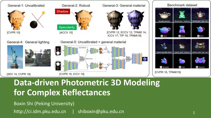
Generalization of photometric stereo Benchmark dataset General-1: Uncalibrated General-2: Robust General-3: General material Shadow Specularity [CVPR 12, ECCV 12, TPAMI 14, [CVPR 10] [ACCV 10] ICCV 17, TIP 19, TPAMI19] General-5: Uncalibrated + general material General-4: General lighting [CVPR 16, TPAMI19] [3DV 14, CVPR 18] [CVPR 19, ICCV 19] 20

Benchmark Datasets and Evaluation 21

“ DiLiGenT ” photometric stereo datasets [Shi 16, 19] https://sites.google.com/site/photometricstereodata Directional Lighting, General reflectance, with ground “ T ruth” shape 22

“ DiLiGenT ” photometric stereo datasets [Shi 16, 19] https://sites.google.com/site/photometricstereodata Directional Lighting, General reflectance, with ground “ T ruth” shape 23

Data capture • Point Grey Grasshopper + 50 mm lens • Resolution: 2448 x 2048 • Object size: 20 cm • Object to camera distance: 1.5 m • 96 white LED in an 8 x 12 grid 24

Lighting calibration Captured image • Intensity 𝑞 𝑘 • Macbeth white balance board • Direction • From 3D positions of LED 𝑺෡ 𝑻 𝑘 + 𝑼 bulbs for higher accuracy 𝑳 −1 𝑞 𝑘 𝒐 𝑄 𝑘 𝒎 𝑘 𝑄 𝑘 Light frame (transformed by ( R , T )) 𝐷 25 Mirror sphere (3D)

“Ground truth” shapes • 3D shape • Scanner: Rexcan CS+ (res. 0.01 mm ) • Registration: EzScan 7 • Hole filling: Autodesk Meshmixer 2.8 • Shape-image registration • Mutual information method [Corsini 09] • Meshlab + manual adjustment • Evaluation criteria • Statistics of angular error (degree) • Mean, median, min, max, 1 st quartile, 3 rd quartile 26

Evaluation for non-Lambertian methods 27

28

Evaluation for non-Lambertian methods • Sort each intensity profile in ascending order • Only use the data ranked between ( T low , T high ) 29

30

Evaluation for uncalibrated methods Opt. A Opt. G Fitting an optimal GBR transform after applying integrability constraint (pseudo-normal up to GBR) 31

32

BALL CAT POT1 BEAR POT2 BUDDHA GOBLET READING COW HARVEST Average 4.10 8.41 8.89 8.39 14.65 14.92 18.50 19.80 25.60 30.62 15.39 BASELINE 2.06 6.73 7.18 6.50 13.12 10.91 15.70 15.39 25.89 30.01 13.35 WG10 Non-Lambertian 2.54 7.21 7.74 7.32 14.09 11.11 16.25 16.17 25.70 29.26 13.74 IW14 3.21 8.22 8.53 6.62 7.90 14.85 14.22 19.07 9.55 27.84 12.00 GC10 2.71 6.53 7.23 5.96 11.03 12.54 13.93 14.17 21.48 30.50 12.61 AZ08 3.55 8.40 10.85 11.48 16.37 13.05 14.89 16.82 14.95 21.79 13.22 HM10 Main dataset 13.58 12.34 10.37 19.44 9.84 18.37 17.80 17.17 7.62 19.30 14.58 ST12 1.74 6.12 6.51 6.12 8.78 10.60 10.09 13.63 13.93 25.44 10.30 ST14 3.34 6.74 6.64 7.11 8.77 10.47 9.71 14.19 13.05 25.95 10.60 IA14 7.27 31.45 18.37 16.81 49.16 32.81 46.54 53.65 54.72 61.70 37.25 AM07 8.90 19.84 16.68 11.98 50.68 15.54 48.79 26.93 22.73 73.86 29.59 SM10 Uncalibrated 4.77 9.54 9.51 9.07 15.90 14.92 29.93 24.18 19.53 29.21 16.66 PF14 4.39 36.55 9.39 6.42 14.52 13.19 20.57 58.96 19.75 55.51 23.92 WT13 3.37 7.50 8.06 8.13 12.80 13.64 15.12 18.94 16.72 27.14 13.14 Opt. A 4.72 8.27 8.49 8.32 14.24 14.29 17.30 20.36 17.98 28.05 14.20 Opt. G 22.43 25.01 32.82 15.44 20.57 25.76 29.16 48.16 22.53 34.45 27.63 LM13 33

Photometric Stereo Meets Deep Learning 34

Photometric stereo + Deep learning • [ICCV 17 Workshop] • Deep Photometric Stereo Network (DPSN) • [ICML 18] • Neural Inverse Rendering for General Reflectance Photometric Stereo (IRPS) • [ECCV 18] • PS-FCN: A Flexible Learning Framework for Photometric Stereo • [ECCV 18] • CNN-PS: CNN-based Photometric Stereo for General Non-Convex Surfaces • [CVPR 19] • Self-calibrating Deep Photometric Stereo Networks (SDPS) • [CVPR 19] • Learning to Minify Photometric Stereo (LMPS) • [ICCV 19] • SPLINE-Net: Sparse Photometric Stereo through Lighting Interpolation and Normal Estimation Networks 35

Photometric stereo + Deep learning Fixed Directions DPSN Unsupervised of Lights IRPS Learning Shadows Global PS-FCN Arbitrary Lights Pixel- CNN-PS BRDFs wisely Uncalibrated SDPS Lights Optimal LMPS Directions Small Number of Lights Arbitrary Features SPLINE-Net Directions 36

[ICCV 17 Workshop] Deep Photometric Stereo Network 37

Research background 𝑔 : reflectance model 𝒏 : measurement vector 𝑴 : light source direction Photometric Stereo 𝒐 : normal vector Image formation Measurements Normal map 𝒏 = 𝑔(𝑴, 𝒐) 𝑴 1 𝑴 2 𝑴 3 𝑴 4 𝑛 1 𝑴 𝟐 𝑜 𝑦 𝑛 2 𝑴 𝟑 𝑜 𝑧 = 𝑔 , 𝑛 3 𝑴 𝟒 𝑜 𝑨 𝑛 4 38 𝑴 𝟓

Motivations Parametric reflectance model Lambertian model (Ideal diffuse reflection) only accurate for a limited class of materials 39 Metal rough surface

Motivations Local illumination model Parametric reflectance model Model direct illumination only Lambertian model (Ideal diffuse reflection) Global illumination effects cannot be modeled only accurate for a limited class of materials 40 Cast shadow Metal rough surface

Motivations Parametric reflectance model Local illumination model • Model the mapping from measurements to surface normal directly using Deep Neural Network (DNN) • DNN can express more flexible reflection phenomenon compared to existing models designed based on physical phenomenon Case shadow Measurements Normal map Deep Neural Network Lambertian model (Ideal diffuse reflection) only accurate for a limited class of materials ∙∙∙ Model direct illumination only Global illumination effects cannot be modeled 41 Metal rough surface

Proposed method Reflectance model with Deep Neural Network T ) • mappings from measurement ( 𝒏 = 𝑛 1 , 𝑛 2 , … , 𝑛 𝑀 T ) to surface normal ( 𝒐 = 𝑜 𝑦 , 𝑜 𝑧 , 𝑜 𝑨 Shadow layer Dense layers 𝑀 images 𝑛 1 𝑛 2 𝑛 3 𝑜 𝑦 𝑛 4 ・・・ 𝑜 𝑧 𝑜 𝑨 ・ ・ ・ ・ ・ ・ ・ ・ ・ 𝑛 𝑀 ・ 42 ・ ・