Nonlinear Dimensionality Visualize all dimensions Visualize the - - PowerPoint PPT Presentation

SLIDE 1

Nonlinear Dimensionality Reduction

Donovan Parks

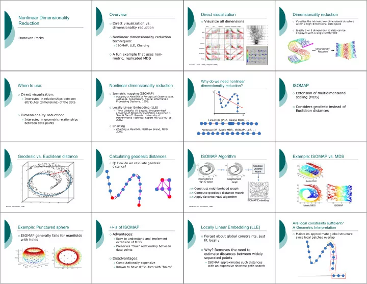
Overview

 Direct visualization vs.

dimensionality reduction

 Nonlinear dimensionality reduction

techniques:

 ISOMAP, LLE, Charting  A fun example that uses non-

metric, replicated MDS

Direct visualization

 Visualize all dimensions

Sources: Chuah (1998), Wegman (1990)

Dimensionality reduction

 Visualize the intrinsic low-dimensional structure

within a high-dimensional data space

 Ideally 2 or 3 dimensions so data can be

displayed with a single scatterplot Dimensionality Reduction

When to use:

 Direct visualization:  Interested in relationships between

attributes (dimensions) of the data

 Dimensionality reduction:  Interested in geometric relationships

between data points

Nonlinear dimensionality reduction

 Isometric mapping (ISOMAP)  Mapping a Manifold of Perceptual Observations.

Joshua B. Tenenbaum. Neural Information Processing Systems, 1998.

 Locally Linear Embedding (LLE)

 Think Globally, Fit Locally: Unsupervised

Learning of Nonlinear Manifolds. Lawrence K. Saul & Sam T. Roweis. University of Pennsylvania Technical Report MS-CIS-02-18, 2002.

 Charting

 Charting a Manifold. Matthew Brand, NIPS

2003.

Why do we need nonlinear dimensionality reduction?

X Y

Linear DR (PCA, Classic MDS, ...) Nonlinear DR (Metric MDS , ISOMAP, LLE, ...)

ISOMAP

 Extension of multidimensional

scaling (MDS)

 Considers geodesic instead of

Euclidean distances

Geodesic vs. Euclidean distance

Source: Tenenbaum, 1998

Calculating geodesic distances

 Q: How do we calculate geodesic

distance?

ISOMAP Algorithm

  Construct neighborhood graph  Compute geodesic distance matrix  Apply favorite MDS algorithm

Geodesic Distance Matrix 1 2 3 Observations in High -D space Neighborhood Graph ISOMAP Embedding

Modified from: Tenenbaum, 1998

Example: ISOMAP vs. MDS Example: Punctured sphere

 ISOMAP generally fails for manifolds

with holes

+/-’s of ISOMAP

 Advantages:  Easy to understand and implement

extension of MDS

 Preserves “true” relationship between

data points

 Disadvantages:  Computationally expensive  Known to have difficulties with “holes”

Locally Linear Embedding (LLE)

 Forget about global constraints, just

fit locally

 Why? Removes the need to

estimate distances between widely separated points

 ISOMAP approximates such distances

with an expensive shortest path search

Are local constraints sufficient? A Geometric Interpretation

 Maintains approximate global structure

since local patches overlap

SLIDE 2

Are local constraints sufficient? A Geometric Interpretation

 Maintains approximate global structure

since local patches overlap

LLE Algorithm

2 ( ) i ij j i j W X W X

• =
• 2

( )

i ij j i j

Y Y W Y

• =
• Source: Saul, 2002

Example: Synthetic manifolds

Modified from: Saul, 2002

Example: Real face images

Source: Roweis, 2000

+/-’s of LLE

 Advantages:  More accurate in preserving local

structure than ISOMAP

 Less computationally expensive than

ISOMAP

 Disadvantages:  Less accurate in preserving global

structure than ISOMAP

 Known to have difficulty on non-convex

manifolds (not true of ISOMAP)

Charting

 Similar to LLE in that it considers

• verlapping “locally linear patches”

(called charts in this paper)

 Based on a statistical framework

instead of geometric arguments

Charting the data

 Place Gaussian at each point and estimate

covariance over local neighborhood

 Brand derives method for

determining optimal covariances in the MAP sense

 Enforces certain constraints to ensure nearby Gaussians (charts) have similar covariance matrices

Find local coordinate systems

 Use PCA in each chart to determine local

coordinate system

Local Coordinate Systems

Connecting the charts

 Exploit overlap of each

neighborhood to determine how to connect the charts

 Brand suggest a

weighted least squares problem to minimize error in the projection of common points

Embedded Charts

Example: Noisy synthetic data

Source: Brand, 2003

+/-’s of Charting

 Advantage:  More robust to noise than LLE or

ISOMAP

 Disadvantage:  More testing needed to demonstrate

robustness to noise

 Unclear computational complexity

 Final step is quadratic in the number of

charts

Conclusion: +/-’s of dimensionality reduction

 Advantages:  Excellent visualization of relationship

between data points

 Limitations:  Computationally expensive  Need many observations  Do not work on all manifolds

Action Synopsis: A fun example

 Action Synopsis: Pose Selection and Illustration.

Jackie Assa, Yaron Caspi, Daniel Cohen-Or. ACM Transactions on Graphics, 2005.

Source: Assa, 2005

Aspects of motion

 Input: pose of person at each frame  Aspects of motion:

 Joint position  Joint angle  Joint velocity  Joint angular velocity Source: Assa, 2005

Dimensionality reduction

 Problem: How can these aspects of motion

be combined?

 Solution: non-metric, replicated MDS

 distance matrix for each aspect of motion  best preserves rank order of distances across

several distance matrices

 Essentially NM-RMDS implicitly weights

each distance matrix

Source: Assa, 2005

Pose selection

 Problem: how do you select

interesting poses from the “motion curve”?

 Typically 5-9 dimensions

 Assa et al. argue that

interesting poses occur at “locally extreme points”

Source: Assa, 2005

SLIDE 3

Finding locally extreme points

Source: Assa, 2005

Do you need dimensionality reduction?

Source: Assa, 2005

Example: Monkey bars

Source: Assa, 2005

Example: Potential application

Source: Assa, 2005

Critique of Action Synopsis

Pros: + Results are convincing + Justified algorithm with user study Cons:

• Little justification for selected aspects of

motion

• Requiring pose information as input is

restrictive

• Unclear that having RMDS implicitly

weight aspects of motion is a good idea

Literature

 Papers covered:  Mapping a Manifold of Perceptual Observations. Joshua B. Tenenbaum. Neural Information Processing Systems, 1998.  Think Globally, Fit Locally: Unsupervised Learning of Nonlinear

• Manifolds. Lawrence Saul & Sam Roweis. University of Pennsylvania

Technical Report MS-CIS-02-18, 2002.  Charting a Manifold. Matthew Brand, NIPS 2003.  Action Synopsis: Pose Selection and Illustration. Jackie Assa, Yaron Caspi, Daniel Cohen-Or. ACM Transactions on Graphics, 2005.  Additional reading:  Multidimensional scaling. Forrest W. Young. Forrest.psych.unc.edu/teaching/p208a/mds/mds.html  A Global Geometric Framework for Nonlinear Dimensionality

• Reduction. Joshua B. Tenenbaum, Vin de Silva, John C. Langford,

Science, v. 290 no.5500, 2000.  Nonlinear dimensionality reduction by locally linear embedding. Sam Roweis & Lawrence Saul. Science v.290 no.5500, 2000.  Further citations:  Information Rich Glyphs for Software Management. M.C. Chuah and S.G. Eick, IEEE CG&A 18:4 1998.  Hyperdimensional Data Analysis Using Parallel Coordinates. Edward J.

• Wegman. Journal of the American Statistical Association, Vol. 85, No.
• 411. (Sep., 1990), pp. 664-675.