[PPT] - Level Set Methods Level Set Methods Contour evolution method PowerPoint Presentation

SLIDE 1

1

Level Set Methods Level Set Methods

Contour evolution method due to J.

Contour evolution method due to J. Sethian Sethian and and S.

S. Osher

Osher, 1988 , 1988

www.math.berkeley.edu/~sethian/level_set.html

www.math.berkeley.edu/~sethian/level_set.html

Difficulties with snake

Difficulties with snake-

type methods

type methods

Hard to keep track of contour if it self

Hard to keep track of contour if it self-

intersects

intersects during its evolution during its evolution

Hard to deal with changes in topology

Hard to deal with changes in topology

The level set approach:

The level set approach:

Define problem in 1 higher dimension

Define problem in 1 higher dimension

Define level set function

Define level set function z = = φ φ φ φ φ φ φ φ( (x,y,t = 0) = 0) where the ( where the (x,y) plane contains the contour, and ) plane contains the contour, and z = signed Euclidean distance transform value = signed Euclidean distance transform value (negative means inside closed contour, positive (negative means inside closed contour, positive means outside contour) means outside contour)

How to Move the Contour? How to Move the Contour?

Move the level set function,

Move the level set function, φ φ φ φ φ φ φ φ( (x,y,t), so that it ), so that it rises, falls, expands, etc. rises, falls, expands, etc.

Contour = cross section at

Contour = cross section at z = 0, i.e., = 0, i.e., {( {(x x, ,y y) | ) | φ φ( (x x, ,y y, ,t t) = 0} ) = 0}

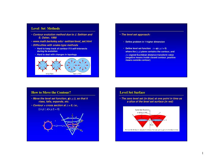
Level Set Surface Level Set Surface

The zero level set (in blue) at one point in time as

The zero level set (in blue) at one point in time as a slice of the level set surface (in red) a slice of the level set surface (in red)

SLIDE 2

2

Level Set Surface Level Set Surface

Later in time the level set surface (red) has

Later in time the level set surface (red) has moved and the new zero level set (blue) moved and the new zero level set (blue) defines the new contour defines the new contour

Level Set Surface Level Set Surface How to Move the Level Set Surface? How to Move the Level Set Surface?

1.

1. Define a velocity field,

Define a velocity field, F, that specifies how , that specifies how contour points move in time contour points move in time

Based on application

Based on application-

specific physics such as time,

specific physics such as time, position, normal, curvature, image gradient position, normal, curvature, image gradient magnitude magnitude

2.

2. Build an initial value for the level set function,

Build an initial value for the level set function, φ φ( (x,y,t=0) =0), based on the initial contour position , based on the initial contour position 3.

3. Adjust

Adjust φ φ over time; contour at time

ver time; contour at time t

t defined by defined by φ φ( (x(t), y(t), t) = 0 ) = 0

y

x
F

t

F

t

2

1 2 2

=

∂

∂ +

∂

∂ + ∂ ∂ = ∇ ⋅ + ∂ ∂

Hamilton

Hamilton-

Jacobi

Jacobi equation equation

Level Set Formulation Level Set Formulation

Constraint: level set value of a point on the contour with

Constraint: level set value of a point on the contour with motion motion x x( (t t) must always be 0 ) must always be 0 φ φ( (x x( (t t), ), t t) = 0 ) = 0

By the chain rule

By the chain rule

φ φt

t +

+ ∇ ∇φ φ( (x x( (t t), ), t t) ) · · x x′ ′( (t t) = 0 ) = 0

Since F supplies the speed in the outward normal direction

Since F supplies the speed in the outward normal direction

x x′ ′( (t t) ) · · n n = = F F, where , where n n = = ∇ ∇φ φ / | / |∇ ∇φ φ| |

Hence evolution equation for

Hence evolution equation for φ φ φ φ φ φ φ φ is is φ φt

t +

+ F F| |∇ ∇φ φ| = 0 | = 0

SLIDE 3

3

Speed Function Speed Function

( )

k

1 (k) F F F(k)

1

− = + =

( ) ( )

✁

k 1 x,y k F(k)

I

− ∗ =

( )

x,y I G

I

✂

I

✄

e k x,y I G 1 1 k

∗ ∇

= ∗ ∇ + =

Example: Shape Simplification Example: Shape Simplification

F = 1

= 1 – – 0.1 0.1κ κ κ κ κ κ κ κ where where κ κ κ κ κ κ κ κ is the curvature at each is the curvature at each contour point contour point

Example: Segmentation Example: Segmentation

Digital Subtraction Angiogram

Digital Subtraction Angiogram

F based on image gradient and contour curvature

based on image gradient and contour curvature

Example (cont.) Example (cont.)

Initial contour specified manually

Initial contour specified manually

SLIDE 4

4

More Examples More Examples More Examples More Examples More Examples More Examples Fast Marching Method Fast Marching Method

J.
J. Sethian

Sethian, 1996 , 1996

Special case that assumes the velocity field,

Special case that assumes the velocity field, F, , never changes sign. That is, contour is either never changes sign. That is, contour is either always expanding ( always expanding (F>0 F>0) or always shrinking ( ) or always shrinking (F<0 F<0) )

Convert problem to a stationary formulation on a

Convert problem to a stationary formulation on a discrete grid where the contour is guaranteed to discrete grid where the contour is guaranteed to cross each grid point at most once cross each grid point at most once

SLIDE 5

5

Fast Marching Method Fast Marching Method

Compute

Compute T( (x,y) = time at which the contour ) = time at which the contour crosses grid point ( crosses grid point (x,y) )

At any height,

At any height, t t, the surface gives the set of , the surface gives the set of points reached at time points reached at time t t

Fast Marching Algorithm Fast Marching Algorithm

Compute T using the fact that

Compute T using the fact that

Distance

Distance = = rate rate × × time time

In 1D: 1 =

In 1D: 1 = F F × × d dT T/ /d dx x

In 2D: 1 =

In 2D: 1 = F F × × | | ∇ ∇ ∇ ∇ ∇ ∇ ∇ ∇T T | |

Contour at time

Contour at time t t = = {( {(x x, ,y y) | ) | T T( (x x, ,y y) = ) = t t} }

Fast Marching Algorithm Fast Marching Algorithm

Construct the arrival time surface

Construct the arrival time surface T( (x,y) ) incrementally: incrementally:

1.

1. Build the initial contour

Build the initial contour 2.

2. Incrementally add on to the existing surface the part

Incrementally add on to the existing surface the part that corresponds to the contour moving with speed that corresponds to the contour moving with speed F (in other words, repeatedly pick a point on the fringe (in other words, repeatedly pick a point on the fringe with minimum with minimum T value) value) 3.

3. Iterate until

Iterate until F goes to 0 goes to 0

Builds level set surface by “scaffolding” the

Builds level set surface by “scaffolding” the surface patches farther and farther away from surface patches farther and farther away from the initial contour the initial contour

Fast Marching Fast Marching

Update “downwind” (i.e., unvisited neighbors) Compute new possible values

SLIDE 6

6

Fast Marching Fast Marching

Expand point on the fringe with minimum value Update neighbors “downwind”

Fast Marching Fast Marching

Expand point on the fringe with minimum value Update neighbors “downwind”

Fast Marching Visualization Fast Marching Visualization

Fast Marching + Level Set for Shape Recovery Fast Marching + Level Set for Shape Recovery

1.

1. First use the Fast Marching algorithm to obtain

First use the Fast Marching algorithm to obtain “rough” contour “rough” contour 2.

2. Then use the Level Set algorithm to fine tune,

Then use the Level Set algorithm to fine tune, using a few iterations, the results from Fast using a few iterations, the results from Fast Marching Marching

( )

x,y I G

e

F F T

∗ ∇

= = ∇

α

, 1

( ) ( )

x,y I G P(x,y) x,y I G 1 1 k

✁ ✁

I

∗ ∇ − = ∗ ∇ + =

( )

P

✂

K k t

✂

I

= Φ ∇ ⋅ ∇ − ∇ − + ∂ ∂ β ε 1

SLIDE 7

7

Results: Segmentation using Fast Marching Results: Segmentation using Fast Marching

No level set tuning No level set tuning

Results: Vein Segmentation Results: Vein Segmentation

No level set tuning With level set tuning No level set tuning With level set tuning

Results: Vein Segmentation (continued) Results: Vein Segmentation (continued)

Original Fast Marching + Original Fast Marching + Level Set only Level Set only Level Set Tuning Level Set Tuning

Results: Segmentation using Fast Marching Results: Segmentation using Fast Marching

No level set tuning No level set tuning

SLIDE 8

8

Results: Brain Image Segmentation Results: Brain Image Segmentation

# of iterations = 9000 # of iterations # of iterations = 9000 # of iterations = 12000 = 12000 Fast marching only, no level set tuning Fast marching only, no level set tuning