1 Volume Graphics - Pros Volume Graphics - Cons Advantages: - - PDF document

1

Volume Rendering

Lecture 21

Slides gathered from Roger Crawfis, Torsten Moeller, Raghu Machiraju, Han-Wei Shen and Ross Whitaker

5/12/2003

• R. Crawfis, Ohio State Univ.

2

Overview

Surface graphics is not enough for ... Introduction to volume graphics Volume rendering techniques

Contour surfaces Ray Casting Cell Projection Splatting

5/12/2003

• R. Crawfis, Ohio State Univ.

3

Surface Graphics

Traditionally, graphics objects are modeled with surface primitives (surface graphics). Continuous in object space

5/12/2003

• R. Crawfis, Ohio State Univ.

4

Difficulty with Surface Graphics

Volumetric object handling

gases, fire, smoke, clouds (amorphous data) sampled data sets (MRI, CT, scientific)

Peeling, cutting, sculpting

any operation that exposes the interior

5/12/2003

• R. Crawfis, Ohio State Univ.

5

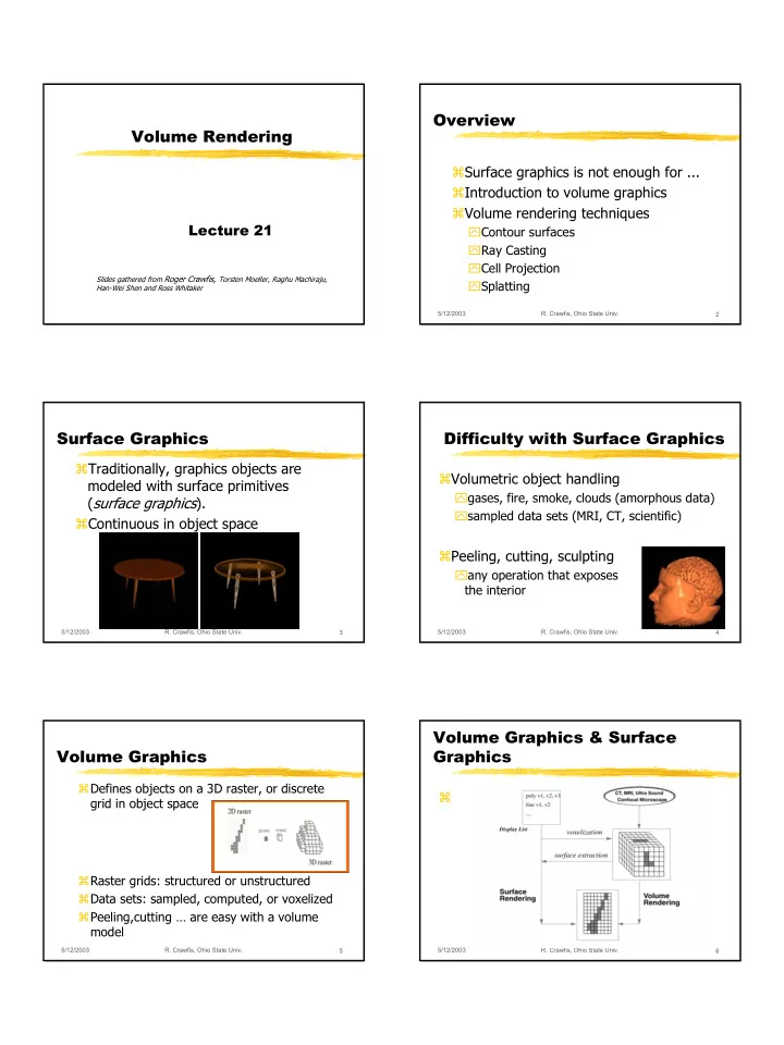
Volume Graphics

Defines objects on a 3D raster, or discrete grid in object space Raster grids: structured or unstructured Data sets: sampled, computed, or voxelized Peeling,cutting … are easy with a volume model

5/12/2003

• R. Crawfis, Ohio State Univ.

6

Volume Graphics & Surface Graphics

2

5/12/2003

• R. Crawfis, Ohio State Univ.

7

Volume Graphics - Cons

Disadvantages: Large memory and processing power Object- space aliasing Discrete transformations Notion of objects is different

5/12/2003

• R. Crawfis, Ohio State Univ.

8

Volume Graphics - Pros

Advantages: Required for sampled data and amorphous phenomena Insensitive to scene complexity Insensitive to surface type Allows block operations

5/12/2003

• R. Crawfis, Ohio State Univ.

9

Volume Graphics Applications (simulation data set)

Scientific data set visualization

5/12/2003

• R. Crawfis, Ohio State Univ.

10

More Volume Graphics Applications (artistic data set)

Amorphous entity visualization

smoke, steam, fire

5/12/2003

• R. Crawfis, Ohio State Univ.

11

Volume Rendering Algorithms

Intermediate geometry based (marching cube) Direct volume rendering

Splatting (forward projection) Ray Casting (backward projection) or resampling Cell Projection / scan-conversion Image warping

5/12/2003

• R. Crawfis, Ohio State Univ.

12

How to visualize?

Slicing: display the volume data, mapped to colors, along a slice plane Iso-surfacing: generate

• paque and semi-opaque

surfaces on the fly Transparency effects: volume material attenuates reflected or emitted light slice Semi-transparent material Iso-surface

3

5/12/2003

• R. Crawfis, Ohio State Univ.

13

Semi -Transparent - How?

Radiative transport theory model the interaction of light with the material

• bserver

light Emission(+) Scattering(+) Absorption(-) Transport of Light

5/12/2003

• R. Crawfis, Ohio State Univ.

14

Semi -Transparent - How?

Rendering Integral (Sabella, Max, …)

( )

( )

∫

α −

=

t t s ds

e s c t I ) (

( )

∫ρ

= α

s t

du u k s ) (

t0 t1 t C(t): shade α(t): opacity ρ(t): “density” Discretize Integral!!

5/12/2003

• R. Crawfis, Ohio State Univ.

15

Solution of Integral

Numerically! I.e. discretize rendering integral replace integral with a Riemann sum Iterative integral evaluation - “over” operator difference: Front-To-Back and Back-To-Front

5/12/2003

• R. Crawfis, Ohio State Univ.

16

Evaluation = Compositing

“over” operator - Porter & Duff 1984

C(N)out Cin Cout C, α Ci, αi C(0)in

α ⋅ + α − ⋅ = C C C

in

• ut

) 1 (

( ) ( )out

in

i C i C 1 − =

5/12/2003

• R. Crawfis, Ohio State Univ.

17

Compositing: Over Operator

cb = (1,0,0) ab = 0.9 cf = (0,1,0) af = 0.4

c = af*cf + (1 - af)*ab*cb a = af + (1 - af)*ab

c = (0.54,0.4,0) a = 0.94

5/12/2003

• R. Crawfis, Ohio State Univ.

18

Direct Rendering Pipeline I

Detection of Structures Shading Reconstruct (interpolate/filter) color/opacity Composite Final Image Validation (change parameters)

4

5/12/2003

• R. Crawfis, Ohio State Univ.

19

Direct Rendering Pipeline II

For continuous media or functions without interfaces, such as temperature:

Reconstruct (interpolate/filter) color/opacity Composite Final Image Validation (change parameters)

5/12/2003

• R. Crawfis, Ohio State Univ.

20

Direct Rendering Pipeline III

Better yet, reconstruct the function and delay the classification until after the resampling:

Reconstruct (interpolate/filter) function values. Apply the transfer function or color table to each sample Composite Final Image Validation (change parameters)

5/12/2003

• R. Crawfis, Ohio State Univ.

21

Direct Rendering Pipeline

Classify Shade Visibility

• rder

Reconstruct Composite Validate

5/12/2003

• R. Crawfis, Ohio State Univ.

22

• Vs. Surface Graphics

Transformation - similar, however some

• ptimizations possible (shearing)

Classification - similar for scalar data, new concepts needed for vector/multi-modal data Interpolation - similar, plus accuracy issues of discretization of the rendering integral Shading - similar concepts for surface effects (diffuse, specular) Compositing - novel for transparencies based on rendering integral

5/12/2003

• R. Crawfis, Ohio State Univ.

23

Early Methods

Before 1988 Did not consider transparency did not consider sophisticated light transportation theory were concerned with quick solutions hence more or less applied to binary data

5/12/2003

• R. Crawfis, Ohio State Univ.

24

Back-To-Front - Frieder et al 1985

A viewing algorithm that traverses and renders the scene objects in order of decreasing distance from the observer. Maybe derived from a standard - “Painters Algorithm” 1. 2. 3.

5

5/12/2003

• R. Crawfis, Ohio State Univ.

25

Back-To-Front - Frieder et al 1985

2D

Start traversal at point farthest from the observer, 2 orders Either x or y can be innermost loop If x is innermost, display order will be A, C, B, D

x y A C D B Screen

If y is innermost, display order will be C, A, D, B Both result in the correct image! If voxel (x,y) is (partially) obscured by voxel (x’,y’), then x <= x’ and y <= y’. So project (x,y) before (x’,y’) and the image will be correct

5/12/2003

• R. Crawfis, Ohio State Univ.

26

Back-To-Front - Frieder et al 1985

3D

Axis traversal can still be done arbitrarily, 8 orders Data can be read and rendered as slices Note: voxel projection is NOT in order of strictly decreasing distance, so this is not the painter’s algorithm. Persepctive?

103 203 303 030 311 312 313 303 302 301 300 213 313 003 323 310 323 223 123 023 013 113 331 332 333 320 321 322 333 333 233 133 033 330 032 132 232 332 033 133 233 130 230 330 031 131 231 331

5/12/2003

• R. Crawfis, Ohio State Univ.

27

Ray Tracing

“another” typical method from traditional graphics Typically we only deal with primary rays - hence: ray-casting a natural image-order technique as opposed to surface graphics - how do we calculate the ray/surface intersection??? Since we have no surfaces - we need to carefully step through the volume

5/12/2003

• R. Crawfis, Ohio State Univ.

28

Ray Casting

Since we have no surfaces - we need to carefully step through the volume: a ray is cast into the volume, sampling the volume at certain intervals The sampling intervals are usually equi-distant, but don’t have to be (e.g. importance sampling) At each sampling location, a sample is interpolated / reconstructed from the grid voxels popular filters are: nearest neighbor (box), trilinear (tent), Gaussian, cubic spline Along the ray - what are we looking for?

5/12/2003

• R. Crawfis, Ohio State Univ.

29

Basic Idea of Ray-casting Pipeline

• Data are defined at the corners
• f each cell (voxel)
• The data value inside the

voxel is determined using interpolation (e.g. tri-linear)

• Composite colors and opacities

along the ray path

• Can use other ray-traversal schemes as well

c1 c2 c3

5/12/2003

• R. Crawfis, Ohio State Univ.

30

Ray Traversal Schemes

Depth Intensity Max Average Accumulate First

6

5/12/2003

• R. Crawfis, Ohio State Univ.

31

Ray Traversal - First

Depth Intensity First First: extracts iso-surfaces (again!) done by Tuy&Tuy ’84

5/12/2003

• R. Crawfis, Ohio State Univ.

32

Ray Traversal - Average

Depth Intensity Average Average: produces basically an X-ray picture

5/12/2003

• R. Crawfis, Ohio State Univ.

33

Ray Traversal - MIP

Depth Intensity Max Max: Maximum Intensity Projection used for Magnetic Resonance Angiogram

5/12/2003

• R. Crawfis, Ohio State Univ.

34

Ray Traversal - Accumulate

Depth Intensity Accumulate Accumulate: make transparent layers visible! Levoy ‘88

5/12/2003

• R. Crawfis, Ohio State Univ.

35

Levoy - Pipeline

Acquired values Data preparation Prepared values classification shading Voxel colors Ray-tracing / resampling Ray-tracing / resampling Sample colors compositing Voxel opacities Sample opacities Image Pixels

5/12/2003

• R. Crawfis, Ohio State Univ.

36

Volumetric Ray Integration

color

• pacity
• bject (color, opacity)

1.0

7

5/12/2003

• R. Crawfis, Ohio State Univ.

37

Interpolation Kernels

color

• pacity
• bject (color, opacity)

1.0

volumetric compositing

5/12/2003

• R. Crawfis, Ohio State Univ.

38

Interpolation Kernels

color

• pacity
• bject (color, opacity)

interpolation kernel

1.0

volumetric compositing color c = c s αs(1 - α) + c

• pacity α = α s (1 - α) + α

5/12/2003

• R. Crawfis, Ohio State Univ.

39

Interpolation Kernels

color

• pacity
• bject (color, opacity)

1.0

volumetric compositing

interpolation kernel

5/12/2003

• R. Crawfis, Ohio State Univ.

40

Interpolation Kernels

color

• pacity
• bject (color, opacity)

1.0

volumetric compositing

5/12/2003

• R. Crawfis, Ohio State Univ.

41

Interpolation Kernels

color

• pacity
• bject (color, opacity)

1.0

volumetric compositing

5/12/2003

• R. Crawfis, Ohio State Univ.

42

Interpolation Kernels

color

• pacity
• bject (color, opacity)

1.0

volumetric compositing

8

5/12/2003

• R. Crawfis, Ohio State Univ.

43

Interpolation Kernels

color

• pacity
• bject (color, opacity)

1.0

volumetric compositing

5/12/2003

• R. Crawfis, Ohio State Univ.

44

Interpolation Kernels

color

• pacity
• bject (color, opacity)

volumetric compositing

5/12/2003

• R. Crawfis, Ohio State Univ.

45

Levoy - Pipeline

Acquired values Data preparation Prepared values classification shading Voxel colors Ray-tracing / resampling Ray-tracing / resampling Sample colors compositing Voxel opacities Sample opacities Image Pixels

5/12/2003

• R. Crawfis, Ohio State Univ.

46

Ray Marching

Use a 3D DDA algorithm to step through regular or rectilinear grids.

5/12/2003

• R. Crawfis, Ohio State Univ.

47

Levoy - Interpolation

eye image pixel viewing ray voxel sample point trilinear interpolation 5/12/2003

• R. Crawfis, Ohio State Univ.

48

Levoy - Interpolation (2)

binary smooth

Closest value Weighted average

9

5/12/2003

• R. Crawfis, Ohio State Univ.

49

Adaptive Ray Sampling

[Hanrahan et al 92]

Sampling rate is adjusted to the significance

• f the traversed data

5/12/2003

• R. Crawfis, Ohio State Univ.

50

Levoy - Derivatives

Central difference per voxel

2 2 2

1 , , 1 , , , 1 , , 1 , , , 1 , , 1 − + − + − +

− = − = − =

k j i k j i z k j i k j i y k j i k j i x

v v G v v G v v G

5/12/2003

• R. Crawfis, Ohio State Univ.

51

Gradient

∇f

∇f = (dx, dy, dz)

• = ( (f(1,0,0) - f(-1,0,0))/2, (f(0,1,0) - f(0,-1,0))/2, (f(0,0,1) - f(0,0,-1))/2)

Approximates "surface normal“ (of isosurface)

5/12/2003

• R. Crawfis, Ohio State Univ.

52

Image Order

Render image one pixel at a time

For each pixel ...

• cast ray
• interpolate
• transfer function
• composite

5/12/2003

• R. Crawfis, Ohio State Univ.

53

Raycasting

Back to Front

straightforward use of over operator intuitively backwards

Front to Back

intuitively right not simple over operator facilitates early ray termination

5/12/2003

• R. Crawfis, Ohio State Univ.

54

Raycasting: compositing

Back to Front:

Ci ; Ai ci ; ai Ci+1 ; Ai+1

Ci+1 = ai*ci + (1 - ai)*Ai*Ci Ai+1 = ai + (1 - ai)*Ai

(eye)

composite order

10

5/12/2003

• R. Crawfis, Ohio State Univ.

55

Raycasting: compositing

Front to Back:

Ci ; Ai ci ; ai Ci+1 ; Ai+1

Ci+1 = Ai*Ci + (1 - Ai)*ai*ci Ai+1 = Ai + (1 - Ai)*ai

(eye)

composite order

5/12/2003

• R. Crawfis, Ohio State Univ.

56

Levoy - Shading

Phong Shading + Depth Cueing

( ) ( ) ( ) ( )

) ) ( ) ( (

2 1 n s d p a p

H x N k L x N k x d k k C k C x C ⋅ + ⋅ + + =

Cp = color of parallel light source ka / kd / ks = ambient / diffuse / specular light coefficient k1, k2 = fall-off constants d(x) = distance to picture plane L = normalized vector to light H = normalized vector for maximum highlight N(xi) = surface normal at voxel xi

5/12/2003

• R. Crawfis, Ohio State Univ.

57

Levoy - Pipeline

Acquired values Data preparation Prepared values classification shading Voxel colors Ray-tracing / resampling Ray-tracing / resampling Sample colors compositing Voxel opacities Sample opacities Image Pixels

5/12/2003

• R. Crawfis, Ohio State Univ.

58

Classification of Scalar Data

Maps raw voxel value into presentable entities: color, intensity, opacity, etc.

• 1. Raw-data → material (R, G, B, α, Ka, Kd, Ks, ...).
• 2. Material → shaded material.

Step 1: may require probabilistic methods (Drebin). Derive material volume from input. Estimate % of each material in all voxels. Pre- computed. Step 2: High gradient in the data values detects surface and is used as a measure of its

• rientation.

5/12/2003

• R. Crawfis, Ohio State Univ.

59

Levoy - Classification

Usually not only interested in a particular iso- surface but also in regions of “change” Feature extraction - High value of opacity exists in regions of change Transfer function (Levoy) - Saliency Surface “strength”

5/12/2003

• R. Crawfis, Ohio State Univ.

60

Levoy

Contour Surfaces with Ray tracing If step is too large, will miss the surface. If step is too small, it is too slow.

L N I I S

11

5/12/2003

• R. Crawfis, Ohio State Univ.

61

Contour Detection

Control step, or iteratively search until you hit the surface. Similar to root finding

5/12/2003

• R. Crawfis, Ohio State Univ.

62

Levoy - Classification

Chemistry Data

• nly iso-value - loose information of layers

iso-range - could be too narrow or too wide thickness of region should be constant hence linear fall off of opacity wider fall off for larger gradient

Medical Data

assume at most two tissues meet linear transition between opacities of “neighboring” tissues reflects linear combination of tissues within one voxel

5/12/2003

• R. Crawfis, Ohio State Univ.

63

Opacity function (1)

Goal: visualize voxels that have a selected threshold value fv

• No intermediate geometry is extracted
• The idea is to assign voxels that have value fv the

maximum opacity (say α)

• And then create a smooth transition for the surrounding

area from 1 to 0

• Levoy wants to maintain a constant thickness for the

transition area.

5/12/2003

• R. Crawfis, Ohio State Univ.

64

Transfer function

“ here’s the edge ” v α v v = f (x) v0 x

5/12/2003

• R. Crawfis, Ohio State Univ.

65

Opacity function (2)

Maintain a constant isosurface thickness

• pacity = α
• pacity = 0

Can we assign opacity based

• n function value instead of

distance? (local operation: we don’t know where the isosurface is) Yes – we can based on the value distance f – fv but we need to take into account the local gradient

5/12/2003

• R. Crawfis, Ohio State Univ.

66

Opacity function (3)

Assign opacity based on value difference (f-fv) and local gradient gradient: the value fall-off rate grad = ∆f/∆s Assuming a region has a constant gradient and the isosurface transition has a thickness R

• pacity = α

F = fv

• pacity = 0

F = fv – grad * R thickness = R F = f(x) Then we interpolate the opacity

• pacity = α – α * ( fv-f(x))/ (grad * R)

12

5/12/2003

• R. Crawfis, Ohio State Univ.

67

Levoy - Classification A

Opacity α(xi) Acquired value f (xi) Gradient magnitude |∇f (xi)| Opacity α(xi) Acquired value f (xi) Gradient magnitude |∇f (xi)|

αv fv

( ) ( ) ( )

        − − α = α

i i v v i

x f x f f r x ' 1 1

5/12/2003

• R. Crawfis, Ohio State Univ.

68

Levoy - Classification B

Opacity α(xi) Acquired value f (xi) Gradient magnitude |∇f (xi)|

αvc αvb αva fva fvb fvc

( ) ( ) ( ) ( )

                − − α +         − − α = α

+ + + + n n n n n n n n

v v i v v v v v i v i i

f f x f f f f f x f x f x

1 1 1 1

'

5/12/2003

• R. Crawfis, Ohio State Univ.

69

"2D" transfer functions

Assign opacity from data value and |∇f| Example of flexibility of volume rendering

5/12/2003

• R. Crawfis, Ohio State Univ.

70

Levoy - Summary

Translation

translates rays vs. data set

Classification

novel, uses gradient

Shading

interpolates colors/opacities vs. normals (gouraud)

Interpolation

tri-linear, central difference

Compositing

image order (ray-casting) back-to-front

5/12/2003

• R. Crawfis, Ohio State Univ.

71

Levoy - Improvements

Levoy 1990 front-to-back with early ray termination α = 0.95 hierarchical oct-tree data structure

skip empty cells efficiently