
SLIDE 1
Regeltechniek
Lecture 11 – State-space models and state feedback control
Robert Babuˇ ska Delft Center for Systems and Control Faculty of Mechanical Engineering Delft University of Technology The Netherlands e-mail: r.babuska@dcsc.tudelft.nl www.dcsc.tudelft.nl/˜babuska tel: 015-27 85117
Robert Babuˇ ska Delft Center for Systems and Control, TU Delft 1
Lecture Outline
Previous lecture: Nyquist plot and stability criterion. (We are finished with frequency domain methods.) Today:
- State-space models, representation.
- State feedback, pole placement.
Robert Babuˇ ska Delft Center for Systems and Control, TU Delft 2
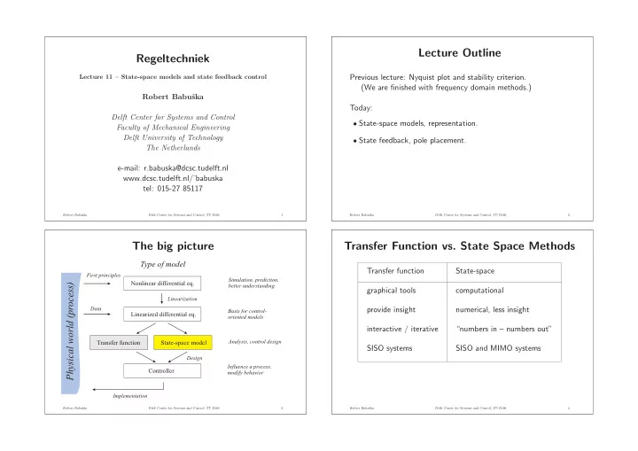
The big picture
Implementation Influenceaprocess, modifybehavior Design
Controller
Analysis,controldesign
State-spacemodel Transferfunction
Data Basisfor
- rientedmodels
control
Linearized differentialeq.
Linearization Simulation,prediction, betterunderstanding
Nonlineardifferentialeq.
Typeofmodel
Firstprinciples
Physicalworld(process)
Robert Babuˇ ska Delft Center for Systems and Control, TU Delft 3
Transfer Function vs. State Space Methods
Transfer function State-space graphical tools computational provide insight numerical, less insight interactive / iterative “numbers in – numbers out” SISO systems SISO and MIMO systems
Robert Babuˇ ska Delft Center for Systems and Control, TU Delft 4