Lecture Outline Systeem- en Regeltechniek II Previous lecture: Bode - - PowerPoint PPT Presentation

SLIDE 1

Systeem- en Regeltechniek II

Lecture 8 – Frequency Domain Design

Robert Babuˇ ska Delft Center for Systems and Control Faculty of Mechanical Engineering Delft University of Technology The Netherlands e-mail: r.babuska@dcsc.tudelft.nl www.dcsc.tudelft.nl/˜babuska tel: 015-27 85117

Robert Babuˇ ska Delft Center for Systems and Control, TU Delft 1

Lecture Outline

Previous lecture: Bode plots, non-minimum-phase systems. Today:

• Bode’s gain-phase relation.
• Neutral stability.
• Gain and phase margin, performance specs.
• Controller design.

Robert Babuˇ ska Delft Center for Systems and Control, TU Delft 2

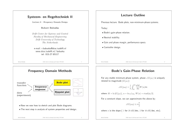
Frequency Domain Methods

frequency response Nyquist plot transfer function

Frequency (rad/sec) Phase (deg); Magnitude (dB) Bode Diagrams

• 40
• 30
• 20
• 10

10

• 1

1 0 0 1 0 1

• 1 5 0
• 1 0 0
• 5 0

data (experiment) Bode plot

• Now we now how to sketch and plot Bode diagrams.
• The next step is analysis of system properties and design.

Robert Babuˇ ska Delft Center for Systems and Control, TU Delft 3

Bode’s Gain-Phase Relation

For any stable minimum-phase system, phase ∠G(jω) is uniquely related to magnitude |G(jω)|: ∠G(jω0) = 1 π ∞

∞

dM du W(u)du where M = ln |G(jω)|, u = ln ω/ω0, W(u) = ctanh|u/2|. For a constant slope, we can approximate the above by: ∠G(jω0) ≃ nπ 2 where n is the slope ( 1 for 20 dB/dec, 2 for 40 dB/dec, etc).

Robert Babuˇ ska Delft Center for Systems and Control, TU Delft 4

SLIDE 2

Consequence of the Gain-Phase Relation

For open loop stable minimum-phase system, it is sometimes suf- ficient to look at the magnitude only. This property can be used to derive a simple design rule for control. But first, we must be able determine, from the Bode plot, whether the system is stable!

Robert Babuˇ ska Delft Center for Systems and Control, TU Delft 5

Bode Plot: Closed-Loop Stability

R s ( )

• +

C s ( ) G s ( ) Y s ( ) U s ( ) E s ( )

L(s) = G(s)C(s) Can we infer closed-loop stability from a Bode plot of the loop transfer function L(s)?

Robert Babuˇ ska Delft Center for Systems and Control, TU Delft 6

Proportional Controller: Loop Transfer

L(s) = Y (s) E(s) = K G(s) For the Bode plot, the following holds: ∠G(jω) = ∠ (KG(jω)) (K is a real number) |G(jω)| = |K| · |G(jω)| (multiplication by a gain) |G(jω)| dB = |K| dB + |G(jω)| dB

Robert Babuˇ ska Delft Center for Systems and Control, TU Delft 7

Proportional Controller: Loop Transfer

10

• 2

10 10

2

10

4

K < 1 K > 1 M a g n i t u d e shift the magnitude response of G(jω) by 20 log(K) phase does not change

Robert Babuˇ ska Delft Center for Systems and Control, TU Delft 8

SLIDE 3

Example: DC Motor

Transfer function: G(s) = θ(s) V (s) = Kt s[(Ls + R)(Js + b) + K2

t ]

inertia of the rotor J = 0.01 kg · m2 damping (friction) b = 0.1 Nms back emf Kt = 0.01 Nm/A resistance R = 1 Ω inductance L = 0.5 H

Robert Babuˇ ska Delft Center for Systems and Control, TU Delft 9

DC Motor: Open-Loop Bode Plot

G(s) = θ(s) V (s) = 2 s(s + 10)(s + 2)

10

−2

10

−1

10 10

1

10

2

−150 −100 −50 50 magnitude (dB) 10

−2

10

−1

10 10

1

10

2

−300 −200 −100 phase (deg) frequency (rad/sec)

Robert Babuˇ ska Delft Center for Systems and Control, TU Delft 10

Influence of Proportional Gain

L(s) = KG(s) = K · 2 s(s + 10)(s + 2) Use Matlab: sisotool(’bode’,G) OK, the magnitude moves up and down with the gain and the phase does not change . . . . . . but, is there anything on the Bode plot that would hint on the stability of the closed loop?

Robert Babuˇ ska Delft Center for Systems and Control, TU Delft 11

Let’s See Whether Root Locus Helps . . .

−12 −10 −8 −6 −4 −2 2 −15 −10 −5 5 10 15 Real Axis Imag Axis

Basic properties of RL: ∠G(s) = −180◦ and |KG(s)| = 1 Neutral stability: |KmaxG(jω)| = 0 dB and ∠G(jω) = −180◦

Robert Babuˇ ska Delft Center for Systems and Control, TU Delft 12

SLIDE 4

Back to the Bode Plot

System is stable if: |KG(jω)| < 0 dB at ∠G(jω) = −180◦

10

−1

10 10

1

10

2

10

3

−200 −100 100 magnitude (dB) 10

−1

10 10

1

10

2

10

3

−300 −200 −100 phase (deg) frequency (rad/sec)

Robert Babuˇ ska Delft Center for Systems and Control, TU Delft 13

Point of Neutral Stability

10

−1

10 10

1

10

2

10

3

−200 −100 100 Kmax|G(jω)| magnitude (dB) 10

−1

10 10

1

10

2

10

3

−300 −200 −100 phase (deg) frequency (rad/sec)

Robert Babuˇ ska Delft Center for Systems and Control, TU Delft 14

Crossover Frequency and Stability Margins

• 150
• 100
• 50

50 10

• 2

10

• 1

10 10

1

10

2

• 300
• 200
• 100

Phase margin Gain margin

Robert Babuˇ ska Delft Center for Systems and Control, TU Delft 15

Crossover Frequency and Stability Margins

• The crossover frequency ωc is the frequency for which the loop

TF has gain 0 dB.

• The gain margin (GM) is the factor (or amount dB) by which

the loop gain can be raised before instability occurs.

• The phase margin (PM) is the amount (in degrees) by which

the phase exceeds 180◦ at ωc.

Robert Babuˇ ska Delft Center for Systems and Control, TU Delft 16

SLIDE 5

Importance of Stability Margins

The margins tell us how far the closed-loop system is from the point of neutral stability. This indicates the robustness w.r.t. un- certainty in the plant model:

• Gain margin: by what factor the total process gain can increase.
• Phase margin: by how much the phase can decrease.

and performance:

• Phase margin: related to closed loop damping (overshoot).
• Crossover frequency: related to response speed

(bandwidth).

Robert Babuˇ ska Delft Center for Systems and Control, TU Delft 17

Robustness: Example

Suppose our model is: ˆ L(s) = 10 s2 + 0.4s + 1 while the true plant is: L(s) = 10 (s2 + 0.4s + 1)(0.1s + 1) Relatively small mismatch in terms of step-response behavior, ma- jor difference in terms of closed-loop stability!

Robert Babuˇ ska Delft Center for Systems and Control, TU Delft 18

Bode Plot of Model and True Plant

−150 −100 −50 50 Magnitude (dB) Bode Diagram Frequency (rad/sec) 10

−1

10 10

1

10

2

10

3

−270 −180 −90 System: G1 Phase Margin (deg): 7.59 Delay Margin (sec): 0.0401 At frequency (rad/sec): 3.3 Closed Loop Stable? Yes Phase (deg) System: G2 Phase Margin (deg): −10.1 Delay Margin (sec): 1.89 At frequency (rad/sec): 3.23 Closed Loop Stable? No

Robert Babuˇ ska Delft Center for Systems and Control, TU Delft 19

Closed-Loop Bandwidth

Bandwidth = frequency up to which the input is “well reproduced” at the output of the closed-loop system. Defined as frequency ωbw at which the magnitude has an attenuation of 0.707 (3dB) – corresponds to 0.5 power gain.

• 3 dB

Magnitude

Robert Babuˇ ska Delft Center for Systems and Control, TU Delft 20

SLIDE 6

Bandwidth and Crossover Frequency

Typically: ωc ≤ ωbw ≤ 2ωc The required speed of response (e.g., the settling time or rise time) can be expressed in terms of ωc. Recall: tr = 1.8/ωn (for second-order dominant response).

Robert Babuˇ ska Delft Center for Systems and Control, TU Delft 21

Phase Margin and Overshoot

The larger PM, the larger damping (less overshoot): ζ ≈ PM 100 this holds up to PM = 60◦ See the Franklin et al. for a graphical relationship between the

• vershoot and PM (page 357).

Robert Babuˇ ska Delft Center for Systems and Control, TU Delft 22

Recall Specs for Second-Order Systems

t t t M e

r n p n s n p

= = − = ± =

− −

18 1 4 6 1%

2 1

2

. . ω π ω ζ ζω

πζ ζ

for

Robert Babuˇ ska Delft Center for Systems and Control, TU Delft 23

More Complex Plants

• System unstable for small K and stable for large K, e.g.,:

L(s) = K(s + 2) s2 − 1

• Conditionally stable systems (unstable for small and large K,

stable for some intermediate values), e.g.,: L(s) = K(s + 2) (s + 10)2(s + 1)(s − 1) In the sequel, we consider systems with no poles in RHP.

Robert Babuˇ ska Delft Center for Systems and Control, TU Delft 24

SLIDE 7

The Basic Idea

• Adjust the proportional gain to get the required crossover fre-

quency and/or steady-state tracking error.

• If needed, use the derivative action to add phase in the neigh-

borhood of ωc in order to increase the phase margin.

• If needed, use the integral action to increase the gain at low fre-

quencies in order to guarantee the required steady-state tracking error.

Robert Babuˇ ska Delft Center for Systems and Control, TU Delft 25

Bode Plots: Homework Assignments

• Read Sections 6.1 through 6.6, except for the Nyquist criterion.
• Work out examples in these sections and verify the results by

using Matlab.

• Reproduce the derivation of the frequency response as given on

the overhead sheets.

• Work out a selection of problems 6.3 through 6.9 and verify

your results by using Matlab.

Robert Babuˇ ska Delft Center for Systems and Control, TU Delft 26