Lecture Outline Regeltechniek Previous lecture: Stability and - - PowerPoint PPT Presentation

Regeltechniek

Lecture 4 – Basics of Feedback Control

Robert Babuˇ ska Delft Center for Systems and Control Faculty of Mechanical Engineering Delft University of Technology The Netherlands e-mail: r.babuska@dcsc.tudelft.nl www.dcsc.tudelft.nl/˜babuska tel: 015-27 85117

Robert Babuˇ ska Delft Center for Systems and Control, TU Delft 1

Lecture Outline

Previous lecture: Stability and transient response. Today:

• Steady-state response.
• Feedforward vs. feedback control.
• Control design goals.
• System type.
• PID control.

Robert Babuˇ ska Delft Center for Systems and Control, TU Delft 2

Steady-State Response

Final value theorem lim

t→∞ y(t) = lim s→0 sY (s)

iff all poles of sY (s) in the LHP If u is a unit step, U(s) = 1

s,

lim

t→∞ y(t) = lim s→0 s · G(s) · 1

s = lim

s→0 G(s)

Consequence: DC (stationary) gain of G(s) DC = lim

s→0 G(s)

Important: G(s) must be stable (check stability first)!

Robert Babuˇ ska Delft Center for Systems and Control, TU Delft 3

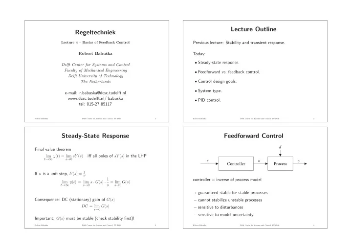
Feedforward Control

d u Controller Process y r controller = inverse of process model + guaranteed stable for stable processes − cannot stabilize unstable processes − sensitive to disturbances − sensitive to model uncertainty

Robert Babuˇ ska Delft Center for Systems and Control, TU Delft 4

Feedback Control

d u Controller Process y r

controller = inverse of process model + can stabilize unstable processes + less sensitive to disturbance + less sensitive to model uncertainty − can potentially destabilize a stable process

Robert Babuˇ ska Delft Center for Systems and Control, TU Delft 5

Feedback vs. Feedforward: Cruise Control

Robert Babuˇ ska Delft Center for Systems and Control, TU Delft 6

Feedback vs. Feedforward: Cruise Control

Controller Car desired speed gas slopewind speed

• Controller

Car desired speed gas slopewind speed

Robert Babuˇ ska Delft Center for Systems and Control, TU Delft 7

Closed-Loop Transfer Function

R s ( )

• +

C s ( ) G s ( ) Y s ( ) U s ( ) E s ( ) Y = GC (R − Y ) (1 + GC) Y = GCR Gcl = Y R = GC 1 + GC

Robert Babuˇ ska Delft Center for Systems and Control, TU Delft 8

Controller Design: Goals and Choices

• Different control goals, for instance:

– stabilize an unstable process – track a specific type of reference signal – reduce influence of disturbances – improve performance (e.g., speed of response)

• Structure of the controller (number of poles and zeros)
• Parameters (location of poles and zeros, gain)

Robert Babuˇ ska Delft Center for Systems and Control, TU Delft 9

Reference Tracking: System Type

R s ( )

• +

C s ( ) G s ( ) Y s ( ) U s ( ) E s ( )

How well will the closed-loop system track a given reference sig- nal? Consider reference input: R(s) = 1 sk k = 1 . . . step, k = 2 . . . ramp, etc.

Robert Babuˇ ska Delft Center for Systems and Control, TU Delft 10

Common Reference Signals

R(s) = 1 s r(t) = 1(t) step (position) R(s) = 1 s2 r(t) = t ramp (velocity) R(s) = 1 s3 r(t) = t2 2 parabola (acceleration)

Robert Babuˇ ska Delft Center for Systems and Control, TU Delft 11

Steady-State Error

R s ( )

• +

C s ( ) G s ( ) Y s ( ) U s ( ) E s ( ) E(s) = 1 1 + L(s)R(s)

with L(s) = G(s)C(s) (loop transfer) Steady-state error (final value theorem): ess = lim

s→0 sE(s) = lim s→0

s 1 + L(s)R(s) = lim

s→0

s 1 + L(s) · 1 sk

Robert Babuˇ ska Delft Center for Systems and Control, TU Delft 12

Steady-State Error: Example 1

Consider the following loop transfer: L(s) = K s + 1 Steady-state error: ess = lim

s→0

s 1 + L(s) · 1 sk = lim

s→0

s(s + 1) s + 1 + K · 1 sk Step (R(s) = 1

s):

ess = lim

s→0

s(s + 1) s + 1 + K · 1 s = 1 1 + K = finite constant Ramp (R(s) = 1

s2):

ess = lim

s→0

s(s + 1) s + 1 + K · 1 s2 = ∞

Robert Babuˇ ska Delft Center for Systems and Control, TU Delft 13

Steady-State Error: Example 2

Consider the following loop transfer: L(s) = K s(s + 1) Steady state error: ess = lim

s→0

s 1 + L(s) · 1 sk = lim

s→0

s2(s + 1) s(s + 1) + K · 1 sk Step (R(s) = 1

s):

ess = lim

s→0

s2(s + 1) s(s + 1) + K · 1 s = 0 Ramp (R(s) = 1

s2):

ess = lim

s→0

s2(s + 1) s(s + 1) + K · 1 s2 = 1 K = finite constant

Robert Babuˇ ska Delft Center for Systems and Control, TU Delft 14

Steady-State Error in General

Loop transfer: L(s) = L0(s) sm ess = lim

s→0

s 1 + L0(s)

sm

· 1 sk = lim

s→0

sms sm + L0(s) · 1 sk Zero steady-state error: ess = 0 iff m ≥ k System type m = number of pure integrators in loop transfer

Robert Babuˇ ska Delft Center for Systems and Control, TU Delft 15

System Type → Controller Structure

If zero steady-state error required (for a given reference type) and the loop transfer is not of sufficiently high type then add integrator(s) in the controller. (see also PID control)

Robert Babuˇ ska Delft Center for Systems and Control, TU Delft 16

Proportional Control

r d u P Process y e

• Controller:
• static gain Kp: u(t) = Kpe(t) = Kp (r(t) − y(t))

Robert Babuˇ ska Delft Center for Systems and Control, TU Delft 17

Closed-Loop Transfer With P Controller

Process (example): G(s) = K s(s + a) Proportional controller: C(s) = Kp Closed-loop poles – solutions of: 1 + KKp s(s + a) = 0 s2 + as + KKp = 0 Kp has some influence on the closed-loop poles (does modify the stiffness, but not the damping)

Robert Babuˇ ska Delft Center for Systems and Control, TU Delft 18

Proportional-Derivative (PD) Control

r d u PD Process y e

• Controller:
• dynamic: u(t) = Kpe(t) + Kd

de(t) dt

• Kp and Kd are the proportional, and derivative gains, respec-

tively

Robert Babuˇ ska Delft Center for Systems and Control, TU Delft 19

Closed-Loop Transfer with PD Controller

Process (example): G(s) = K s(s + a) Proportional controller: C(s) = Kp + Kds Closed-loop poles – solutions of: 1 + K(Kp + Kds) s(s + a) = 0 s2 + (a + KKd)s + KKp = 0 we can choose Kp and Kd to completely determine the closed-loop poles (for this second-order process)

Robert Babuˇ ska Delft Center for Systems and Control, TU Delft 20

PID Control

r d u PID Process y e

• Controller:
• dynamic: u(t) = Kpe(t) + Ki

t

0 e(τ)dτ + Kd de(t) dt

• Kp, Ki and Kd are the proportional, integral and derivative

gains, respectively

Robert Babuˇ ska Delft Center for Systems and Control, TU Delft 21

When Should We Use Integral Action?

If zero steady-state error required (for a given reference type) and the loop transfer is not of sufficiently high type Example: L(s) = G(s)Kp = KKp τs + 1 Reference = step: R(s) = 1 s Required: zero steady-state error ess = 0 Conclusion: as system type is 0 (no integrator), use PI!

Robert Babuˇ ska Delft Center for Systems and Control, TU Delft 22

Integral Action in Differential Equation

Process (example): y + b ˙ y = u Proportional controller: u = Kp(r − y) Closed-loop differential equation: y + b ˙ y = Kpr − Kpy In steady state ( ˙ y = 0): y = Kp 1 + Kp r ⇒ y ≈ r (for large Kp) non-zero steady-state error! (system is of type 0)

Robert Babuˇ ska Delft Center for Systems and Control, TU Delft 23

With a PI Controller

Process (example): y + b ˙ y = u PI controller: u = Kp(r − y) + Ki

• (r − y)

for r =const: ˙ u = −Kp ˙ y + Ki(r − y) Closed-loop differential equation: ˙ y + b¨ y = −Kp ˙ y + Kir − Kiy In steady state (¨ y = ˙ y = 0): 0 = Kir − Kiy ⇒ y = r no steady-state error!

Robert Babuˇ ska Delft Center for Systems and Control, TU Delft 24

Influence of the PID Parameters

• Kp . . . stiffness (speed of response), but also oscillations
• Kd . . . damping (less oscillations), but sensitive to noise
• Ki . . . remove steady-state error, but more overshoot

(re-tune Kp , Ki) Tuning:

• Experimental tuning (often used in practice, sometimes computer-

assisted)

• Model-based analysis and design (rest of our course)

Robert Babuˇ ska Delft Center for Systems and Control, TU Delft 25

Implementation: Computer Control

y(t) u(t)

Computer Process Algorithm Clock { ( )} u t

{ ( )} y t k

k

A-D D-A

Controller implemented on a digital computer, runs in discrete time and on discrete-valued data.

Robert Babuˇ ska Delft Center for Systems and Control, TU Delft 26