
SLIDE 1
Systeem- en Regeltechniek II
Lecture 9 – Lead and Lag Compensators
Robert Babuˇ ska Delft Center for Systems and Control Faculty of Mechanical Engineering Delft University of Technology The Netherlands e-mail: r.babuska@tudelft.nl www.dcsc.tudelft.nl/˜babuska tel: 015-27 85117
Robert Babuˇ ska Delft Center for Systems and Control, TU Delft 1
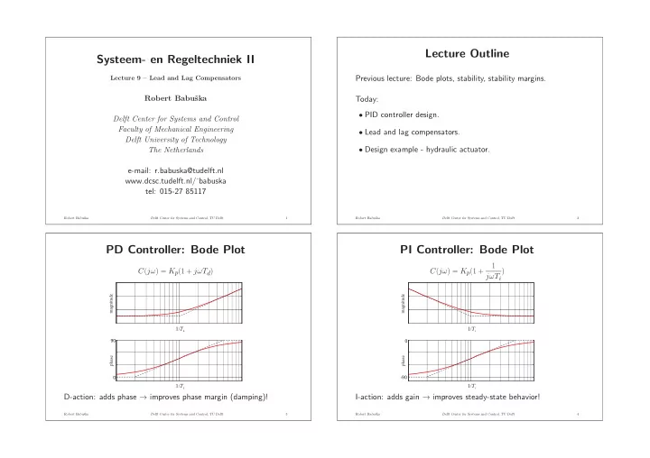
Lecture Outline
Previous lecture: Bode plots, stability, stability margins. Today:
- PID controller design.
- Lead and lag compensators.
- Design example - hydraulic actuator.
Robert Babuˇ ska Delft Center for Systems and Control, TU Delft 2
PD Controller: Bode Plot
C(jω) = Kp(1 + jωTd)
magnitude 90 phase
1/Td 1/Td
D-action: adds phase → improves phase margin (damping)!
Robert Babuˇ ska Delft Center for Systems and Control, TU Delft 3
PI Controller: Bode Plot
C(jω) = Kp(1 + 1 jωTi )
magnitude
- 90
phase
1/Ti 1/Ti
I-action: adds gain → improves steady-state behavior!
Robert Babuˇ ska Delft Center for Systems and Control, TU Delft 4