
SLIDE 1
Systeem- en Regeltechniek II
Lecture 10 – Nyquist plot and stability criterium
Robert Babuˇ ska Delft Center for Systems and Control Faculty of Mechanical Engineering Delft University of Technology The Netherlands e-mail: r.babuska@dcsc.tudelft.nl www.dcsc.tudelft.nl/˜babuska tel: 015-27 85117
Robert Babuˇ ska Delft Center for Systems and Control, TU Delft 1
Lecture Outline
Previous lecture: PID controller design, lead and lag compen- sators. Today:
- Nyquist plot.
- Nyquist stability criterion.
Robert Babuˇ ska Delft Center for Systems and Control, TU Delft 2
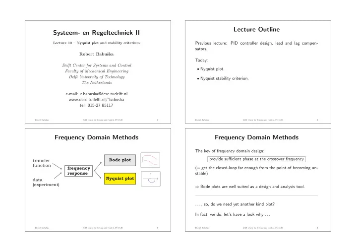
Frequency Domain Methods
frequency response Nyquist plot transfer function
Frequency (rad/sec) Phase (deg); Magnitude (dB) Bode Diagrams- 40
- 30
- 20
- 10
- 1
- 1 5 0
- 1 0 0
- 5 0
data (experiment) Bode plot
Robert Babuˇ ska Delft Center for Systems and Control, TU Delft 3
Frequency Domain Methods
The key of frequency domain design: provide sufficient phase at the crossover frequency (= get the closed-loop far enough from the point of becoming un- stable) ⇒ Bode plots are well suited as a design and analysis tool. . . . , so, do we need yet another kind plot? In fact, we do, let’s have a look why . . .
Robert Babuˇ ska Delft Center for Systems and Control, TU Delft 4