Lecture no: 2 Short on dB calculations Basics about antennas - - PowerPoint PPT Presentation

2010-03-17 Ove Edfors - ETI 051 1

Ove Edfors, Department of Electrical and Information Technology Ove.Edfors@eit.lth.se

RADIO SYSTEMS – ETI 051

Lecture no: 2

Propagation mechanisms

2010-03-17 Ove Edfors - ETI 051 2

Contents

• Short on dB calculations
• Basics about antennas
• Propagation mechanisms

– Free space propagation – Reflection and transmission – Propagation over ground plane – Diffraction

• Screens
• Wedges
• Multiple screens

– Scattering by rough surfaces – Waveguiding

2010-03-17 Ove Edfors - ETI 051 3

DECIBEL

2010-03-17 Ove Edfors - ETI 051 4

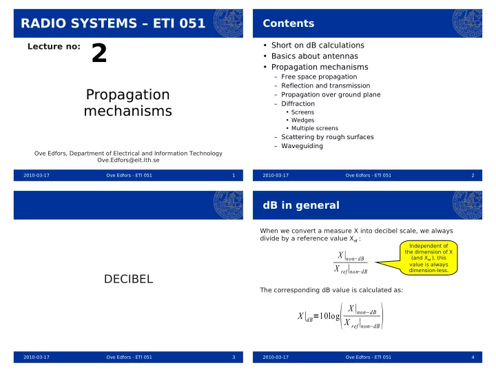
dB in general

X∣dB=10log X∣non−dB X ref∣non−dB

When we convert a measure X into decibel scale, we always divide by a reference value Xr

e f :

X∣non−dB X ref∣non

−dB Independent of the dimension of X (and Xr

e f ), this

value is always dimension-less.

The corresponding dB value is calculated as:

2010-03-17 Ove Edfors - ETI 051 5

Power

We usually measure power in Watt [W] and milliWatt [mW] The corresponding dB notations are dB and dBm Non-dB dB

P∣dB=10log P∣

W

1∣

W =10log P∣W 

Watt:

P∣

W

P∣mW

P∣dBm=10log P∣mW 1∣mW =10logP∣mW

milliWatt:

P∣dBm=10log P∣W 0.001∣W=10 logP∣

W 30∣dB=P∣dB30∣dB

RELATION:

2010-03-17 Ove Edfors - ETI 051 6

Example: Power

GSM mobile TX: 1 W = 0 dB or 30 dBm GSM base station TX: 40 W = 16 dB or 46 dBm Bluetooth TX: 10 mW = -20 dB or 10 dBm Vacuum cleaner: 1600 W = 32 dB or 62 dBm Car engine: 100 kW = 50 dB or 80 dBm ”Typical” TV transmitter: 1000 kW ERP = 60 dB or 90 dBm ERP Sensitivity level of GSM RX: 6.3x10-

1 4 W = -132 dB or -102 dBm

Nuclear powerplant (Barsebäck): 1200 MW = 91 dB or 121 dBm

ERP – Effective Radiated Power

2010-03-17 Ove Edfors - ETI 051 7

Amplification and attenuation

(Power) Amplification:

Pin

G

P out

P out=GPin⇒G= Pout Pin

The amplification is already dimension-less and can be converted directly to dB:

G∣dB=10log

10G

(Power) Attenuation:

Pin

1/L

P out

P out= P in L ⇒ L= Pin Pout

The attenuation is already dimension-less and can be converted directly to dB:

L∣dB=10log10L

Note: It doesn’t matter if the power is in mW or W. Same result!

2010-03-17 Ove Edfors - ETI 051 8

Example: Amplification and attenuation

High frequency cable RG59

1000 2000 3000 4000 5000 20 40 60 80 100 120 140

Frequency [MHz] Attenuation [dB/100m] 30 m of RG59 feeder cable for an 1800 MHz application has an attenuation:

G∣dB=30 L∣dB/100m 100



dB/1m

1800 58

=30 58 100 =17.4

2010-03-17 Ove Edfors - ETI 051 9

Example: Amplification and attenuation

30 dB 10 dB 4 dB 10 dB Detector Ampl. Ampl. Ampl. Cable A B The total amplification of the (simplified) receiver chain (between A and B) is

G A, B∣dB=30−41010=46

2010-03-17 Ove Edfors - ETI 051 10

ANTENNA BASICS

2010-03-17 Ove Edfors - ETI 051 11

The isotropic antenna

The isotropic antenna radiates equally in all directions

Radiation pattern is spherical This is a theoretical antenna that cannot be built. Elevation pattern Azimuth pattern

2010-03-17 Ove Edfors - ETI 051 12

The dipole antenna

Elevation pattern Azimuth pattern

• dipole

λ/2 λ/2

Feed A dipole can be of any length, but the antenna patterns shown are only for the λ/2-dipole. Antenna pattern of isotropic antenna. This antenna does not radiate straight up or

• down. Therefore, more

energy is available in

• ther directions.

THIS IS THE PRINCIPLE BEHIND WHAT IS CALLED ANTENNA GAIN.

2010-03-17 Ove Edfors - ETI 051 13

Antenna gain (principle)

Antenna gain is a relative measure. We will use the isotropic antenna as the reference.

Radiation pattern Isotropic and dipole, with equal input power! Isotropic, with increased input power. The increase of input power to the isotropic antenna, to obtain the same maximum radiation is called the antenna gain!

Antenna gain of the λ/2 dipole is 2.15 dB.

2010-03-17 Ove Edfors - ETI 051 14

Antenna beamwidth (principle)

Radiation pattern The isotropic antenna has ”no”

• beamwidth. It radiates equally

in all directions. The half-power beamwidth is measured between points were the pattern as decreased by 3 dB. 3 dB

2010-03-17 Ove Edfors - ETI 051 15

Receiving antennas

In terms of gain and beamwidth, an antenna has the same properties when used as transmitting or receiving antenna. A useful property of a receiving antenna is its ”effective area”, i.e. the area from which the antenna can ”absorb” the power from an incoming electromagnetic wave. Effective area AR

X of an antenna is

connected to its gain:

GRX= ARX AISO = 4 2 ARX

It can be shown that the effectiva are of the isotropic antenna is:

AISO= 

2

4

Note that AIS

O becomes

smaller with increasing frequency, i.e. with smaller wavelength.

2010-03-17 Ove Edfors - ETI 051 16

A note on antenna gain

Sometimes the notation dBi is used for antenna gain (instead of dB). The ”i” indicates that it is the gain relative to the isotropic antenna (which we will use in this course). Another measure of antenna gain frequently encountered is dBd, which is relative to the λ/2 dipole.

G∣dBi=G∣dBd2.15

Be careful! Sometimes it is not clear if the antenna gain is given in dBi or dBd.

2010-03-17 Ove Edfors - ETI 051 17

EIRP

Effective Isotropic Radiated Power

EIRP = Transmit power (fed to the antenna) + antenna gain

EIRP∣dB=PTX ∣dBGTX ∣dB

Answers the questions: How much transmit power would we need to feed an isotropic antenna to obtain the same maximum on the radiated power? How ”strong” is our radiation in the maximal direction of the antenna?

This is the more important one, since a limit on EIRP is a limit

• n the radiation in the

maximal direction.

2010-03-17 Ove Edfors - ETI 051 18

EIRP and the link budget

EIRP∣

dB=P TX ∣dBG TX ∣dB

”POWER” [dB] Gain Loss

GTX ∣dB

PTX ∣dB

EIRP

2010-03-17 Ove Edfors - ETI 051 19

PROPAGATION MECHANISMS

2010-03-17 Ove Edfors - ETI 051 20

Propagation mechanisms

• We are going to study the fundamental propagation

mechanisms

• This has two purposes:

– Gain an understanding of the basic mechanisms – Derive propagation losses that we can use in calculations

• For many of the mechanisms, we just give a brief
• verview

2010-03-17 Ove Edfors - ETI 051 21

FREE SPACE PROPAGATION

2010-03-17 Ove Edfors - ETI 051 22

Free-space loss Derivation

Assumptions:

Isotropic TX antenna d Distance d

AR

X

RX antenna with effective area AR

X

Received power: P RX= A RX

Atot P TX = ARX 4d

2 P TX

If we assume RX antenna to be isotropic:

TX TX RX

P d P d P

2 2 2

4 4 4 /       = = π λ π π λ

Attenuation between two isotropic antennas in free space is (free-space loss):

L free d = 4 d  

2 Area of sphere:

Atot=4d

2

Relations:

TX power PT

X

PT

X

2010-03-17 Ove Edfors - ETI 051 23

Free-space loss Non-isotropic antennas

Received power, with isotropic antennas (GT

X=GR X =1):

P RX d = PTX L free  d 

Received power, with antenna gains GT

X and GR X :

P RX d =G RXGTX L freed  PTX =G RXGTX



4d  

2 PTX This relation is called Friis’ law

P RX∣dBd =PTX∣dBGTX∣dB−L free∣dBd G RX∣dB =PTX∣dBGTX∣dB−20log10 4d  GRX∣dB

2010-03-17 Ove Edfors - ETI 051 24

Free-space loss Non-isotropic antennas (cont.)

P RX ∣dB  d =PTX ∣dBGTX ∣dB−L free∣dB d G RX∣dB

”POWER” [dB] Gain Loss

Let’s put Friis’ law into the link budget

GTX ∣dB PTX ∣dB GRX ∣dB L free∣dB  d =20log10 4πd λ  P RX ∣dB

How come that the received power decreases with increasing frequency (decre- asing λ)? Does it? Received power decreases as 1/d2, which means a propagation exponent

• f n = 2.

2010-03-17 Ove Edfors - ETI 051 25

Free-space loss Example: Antenna gains

Assume following three free-space scenarios with λ/2 dipoles and parabolic antennas with fixed effective area Ap

a r :

D-D: D-P: P-P: Antenna gains

Gdip∣dB=2.15

G par∣dB=10log10 A par Aiso =10log10 A par 2/4π =10log10 4 Apar 2 

2010-03-17 Ove Edfors - ETI 051 26

Received power increases with decreasing wavelength λ, i.e. with increasing frequency. Received power decreases with decreasing wavelength λ, i.e. with increasing frequency.

Free-space loss Example: Antenna gains (cont.)

Evaluation of Friis’ law for the three scenarios: D-D: P RX ∣dB  d =PTX ∣dB2.15−20 log10 4d  2.15 =PTX ∣dB4.3−20 log10 4d 20log10 D-P: P RX ∣dB  d =PTX ∣dB2.15−20 log10 4 d  10log10 4 Apar 2  =PTX ∣dB2.15−20log10 4d 10log104 A par

P RX ∣dB  d =PTX ∣dB10 log10 4 A par 2 −20log10 4 d  10 log10 4 A par 2  =PTX ∣dB20log10 4A par −20 log10 4 d −20log10 

P-P:

Received power independent of wavelength, i.e. of frequency.

2010-03-17 Ove Edfors - ETI 051 27

Free-space loss Validity - the Rayleigh distance

The free-space loss calculations are only valid in the far field of the antennas. Far-field conditions are assumed ”far beyond” the Rayleigh distance:

d R= 2 La

2



where La is the largest dimesion of the antenna.

• dipole

/2

/2

La=/2 d R=/2

Parabolic

La=2r

d R=8r 2 

2r

Another rule of thumb is: ”At least 10 wavelengths”

2010-03-17 Ove Edfors - ETI 051 28

REFLECTION AND TRANSMISSION

2010-03-17 Ove Edfors - ETI 051 29

Reflection and transmission Snell’s law

I n c i d e n t w a v e R e f l e c t e d w a v e Transmitted wave Θi Θr Θt

{

Θi=Θr sinΘt sinΘi = ε1

 ε2

ε1 ε2 Dielectric constants

2010-03-17 Ove Edfors - ETI 051 30

Reflection and transmission Refl./transm. coefficcients

The property we are going to use: No loss and the electric field is phase shifted 180O (changes sign). Perfect conductor Given complex dielectric constants

• f the materials, we can also

compute the reflection and transmission coefficients for incoming waves of different polarization. [See textbook.]

2010-03-17 Ove Edfors - ETI 051 31

PROPAGATION OVER A GROUND PLANE

2010-03-17 Ove Edfors - ETI 051 32

Propagation over ground plane Geometry

d 180O (π rad) hTX

hRX

d refl Propagation distances: d direct

d direct=d 2hTX−hRX 

2

hRX

d refl=d 2hTXhRX 

2

Δd =d refl−d direct

Phase difference at RX antenna:

Δφ=2π Δd λ π=2π f Δd c 1 2

2010-03-17 Ove Edfors - ETI 051 33

Propagation over ground plane Geometry

What happens when the two waves are combined? Δφ

Attenuated direct wave Attenuated reflected wave

Vector addition of electric fields

( )

d Etot

Taking the free-space propagation losses into account for each wave, the exact expression becomes rather complicated. Finally, after applying an approximation of the phase difference:

L ground  d ≈ 4π d λ 

2



λd 4π hTX hRX 

2

= d 4 hTX

2 hRX 2

Assuming equal free-space attenuation

• n the two waves we get:

∣E tot d ∣=∣E  d ∣×∣1e jΔφ∣

Free space attenuated Extra attenuation Approximation valid beyond:

d limit≥ 4hTX hRX λ

2010-03-17 Ove Edfors - ETI 051 34

Propagation over ground plane Non-isotropic antennas

P RX ∣dB  d =PTX ∣dBGTX ∣dB−Lground∣dB d G RX∣dB

”POWER” [dB] Gain Loss

Let’s put Lg

r

• u

n d into the link budget

GTX ∣dB PTX ∣dB GRX ∣dB

L ground∣dB  d =20log10 d 2 hTX hRX 

P RX ∣dB

There is no frequency dependence on the propagation attenuation, which was the case for free space. Received power decreases as 1/d4, which means a propagation exponent

• f n = 4.

2010-03-17 Ove Edfors - ETI 051 35

Rough comparison to ”real world”

Received power [log scale] Distance, d

TX RX

∝1/d 2 ∝1/d 4

Free space Ground

d limit

We have tried to explain ”real world” propagation loss using theoretical models. In the ”real world” there is one more breakpoint, where the received power decreases much faster than 1/d4.

2010-03-17 Ove Edfors - ETI 051 36

Rough comparison to ”real world” (cont.)

hT

X {

} hR

X

dh

Optic line-of-sight One thing that we have not taken into account: Curvature of earth!

d h≈4.1hTX ∣m hRX∣m∣km

An approximation of the radio horizon: beyond which received power decays very rapidly.

2010-03-17 Ove Edfors - ETI 051 37

DIFFRACTION

2010-03-17 Ove Edfors - ETI 051 38

Diffraction Absorbing screen

Shadow zone

Huygen’s principle

A b s

• r

b i n g s c r e e n

2010-03-17 Ove Edfors - ETI 051 39

Diffraction Absorbing screen (cont.)

For the case of one screen we have exact solutions or good approximations Maybe this is a good solution for predicting propagation

• ver roof-tops?

2010-03-17 Ove Edfors - ETI 051 40

Diffraction Approximating buildnings

There are no solutions for multiple screens, except for very special cases! Several approximations

• f varying quality

exist. [See textbook]

2010-03-17 Ove Edfors - ETI 051 41

Diffraction Wedges

Dielectric wedge Reasonably simple far-field approximations exist. Can be used to model terrain or obstacles

2010-03-17 Ove Edfors - ETI 051 42

SCATTERING BY ROUGH SURFACES

2010-03-17 Ove Edfors - ETI 051 43

Scattering by rough surfaces Scattering mechanism

Smooth surface Specular reflection Scattering Rough surface Specular reflection Due to the ”roughness” of the surface, some of the power of the specular reflection lost and is scattered in other directions.

Two main theories exist: Kirchhoff and pertubation. Both rely on statistical descriptions of the surface height.

2010-03-17 Ove Edfors - ETI 051 44

WAVEGUIDING

2010-03-17 Ove Edfors - ETI 051 45

Waveguiding

Street canyons, corridors & tunnels

Conventional waveguide theory predicts exponential loss with distance. The waveguides in a radio environment are different:

• Lossy materials
• Not continuous walls
• Rough surfaces
• Filled with metallic and

dielectric obstacles Majority of measurements fit the 1/dn law.

2010-03-17 Ove Edfors - ETI 051 46

Summary

• Some dB calculations
• Antenna gain and effective area.
• Propagation in free space, Friis’ law and

Rayleigh distance.

• Propagation over a ground plane.
• Diffraction
• Screens
• Wedges
• Multiple screens
• Scattering by rough surfaces
• Waveguiding