LECTURE 3 Large LECTURE 3 Medium Small How does f change - - PowerPoint PPT Presentation

CTEQ-MCnet school on QCD Analysis and Phenomenology and the Physics and Techniques of Event Generators

Lauterbad (Black Forest), Germany 26 July - 4 August 2010 Introduction to the Parton Model and Perturbative QCD Fred Olness (SMU)

LECTURE 3 LECTURE 3

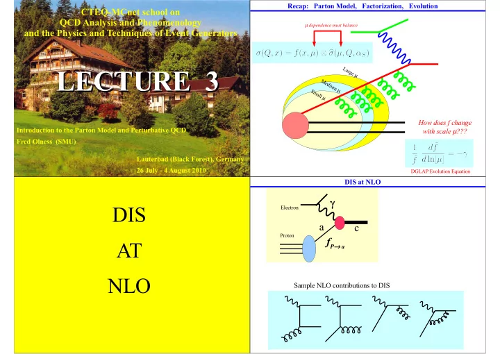
Recap: Parton Model, Factorization, Evolution

Large µ Medium µ Small µ

How does f change with scale µ???

µ dependence must balance

DGLAP Evolution Equation

DIS AT NLO

DIS at NLO

fP→ a a

Electron Proton

γ c

Sample NLO contributions to DIS

DIS NLO Kinematics

θ

q=k1 p=k2 k3 k4

Mandelstam Variables {s,t,u}

{s,t,u} are partonic 1 2 3 4 1 2 3 4 1 2 3 4

s t u

Exercise

p1 = E1 ,0 ,0 , p p1

2=m1 2

p2 = E2 ,0 ,0 ,− p p2

2=m2 2

p1 p2

E1,2 =  s±m1

2∓m2 2

2  s p =  s ,m1

2,m2 2

2  s

a ,b ,c = a

2b 2c 2−2abbcca

1) Let's work out the general 2→2 kinematics for general masses.

a) Start with the incoming particles. Show that these can be written in the general form: ... with the following definitions: Note that ∆(a,b,c) is symmetric with respect to its arguments, and involves the only invariants of the initial state: s, m1

2, m2 2.

b) Next, compute the general form for the final state particles, p3 and p4. Do this by first aligning p3 and p4 along the z-axis (as p1 and p2 are), and then rotate about the y-axis by angle θ.

Homework

p1 p4 p3 p2

θ Homework Part 2

Hint: by using invariants you can keep it simple. I.e., don't do it the way Goldstein does. The power of invariants

p1 p4 p3 p2

θ

Matrix element: NLO DIS Singular at z=1 Singular at x=1 Collinear Singularity Soft Singularity

For the real 2→2 graphs

Separate infinity, absorb in PDF

Separate infinity, cancel with virtual graphs

The Plan

Collinear Divergences Plan Choices Method 1) Separate ∞ at z=1 2) “Absorb” into PDF Need to regulate ∞ 1) Dimensional Regularization 2) Quark Mass 3) θ Cut

Looks like a PDF splitting function

Soft Singularities Plan Choices Method 1) Separate ∞ at x=1 2) Cancel between Real and Virtual graphs Need to regulate ∞ 1) Dimensional Regularization 2) Gluon Mass 3) ...

Dimensional Regularization meets Freshman E&M

• M. Hans, Am.J.Phys. 51 (8) August (1983). p.694
• C. Kaufman, Am.J.Phys. 37 (5), May (1969) p.560
• B. Delamotte, Am.J.Phys. 72 (2) February (2004) p.170

Regularization, Renormalization, and Dimensional Analysis: Dimensional Regularization meets Freshman E&M. Olness & Scalise, arXiv:0812.3578 [hep-ph]

We'll use a simple example to illustrate the key points: y x r dV = 1 40 dQ r

V =  40 ∫

−∞ ∞

dy 1

x

2 y 2= ∞

Infinite Line of Charge Note: ∞ can be very useful r= x

2y 2

=Q/ y V kx= =  40 ∫

−∞ ∞

dy 1

kx

2y 2

=  40 ∫

−∞ ∞

d y k  1

 x

2 y/k  2

=  40 ∫

−∞ ∞

dz 1

 x

2z 2

=V x Scale Invariance

V kx=V x

y x r Note: ∞ + c = ∞ ∴ ∞ ∴ ∞ - ∞ = ∞ = c

How do we distinguish this from

∞ ∞ - ∞ = = c+17 Naively Implies: V(kx) – V(x) = 0 Problem solved at the expense of an extra scale L AND we have a broken symmetry: translation invariance V =  40 ∫

−L L

dy 1

 x

2 y 2

V =  40 log[ L L

2x 2

−L L

2x 2]

E x=−dV dx =  20 x L

 L

2x 2 

 20 x V =V x1−V  x2  L∞  40 log[ x2

2

x1

2]

Cutoff Method V(x) depends on artificial regulator L We cannot remove the regulator L All physical quantities are independent of the regulator:

Electric Field Energy

V =  40 ∫

−Lc Lc

dy 1

 x

2y 2

V =  40 log[ LcLc

2x 2

−L−cL−c

2x 2]

Broken Translational Symmetry y x r +L

• L

Shift: y → y' = y – c y=[+L+c, -L+c] V(r) depends on “y” coordinate!!!

In QFT, gauge symmetries are important. E.g., Ward identies

Dimensional Regularization dy d

n y=d n

2 y

n−1dy

V =  40 ∫0

∞

d n y

n−1



n−1

dy

 x

2 y 2

n=∫ d n= 2

n/2

n/2 1,2,3,4={2,2 ,4 ,2

2}

V =  40  

2

x

2

[] 

 

Compute in n-dimensions

New scale µ Each term is individually dimensionaless

y x r dV = 1 40 dQ r

V =  40 f x

Why do we need an extra scale µ µ ??? r= x

2y 2

=Q/ y Dimensional Regularization E x=−dV dx =  40 [ 2

2 []



 x 12 ]

 0  20 1 x V =V x1−V  x2   0  40 log[ x2

2

x1

2]

Problem solved at the expense of an extra scale µ AND regulator ε Translation invariance is preserved!!! All physical quantities are independent of the regulators:

Electric Field Energy

Dimensional Regularization respects symmetries

Renormalization V   40 [ 1 ln[ e

−E

 ]ln[ 

2

x

2]]

V MS x1−V MSx2=V =V MSx1−V MSx2 V MS x1−V MSx2≠V ≠V MS x1−V MS x2 V   40 [ 1  ln[ e

−E

 ]ln[ 

2

x

2]]

V   40 [ 1 ln[ e

−E

 ]ln[ 

2

x

2]]

Original MS-Bar MS Physical quantities are independent of renormalization scheme! But only if performed consistently:

Connection to QFT V   40 [ 1 ln[ e

−E

1 ]ln[ 

2

x

2]]

D  =  4

2

Q

2 

1− 1−2  [ 1 ln[ e

−E

4 ]ln[ 

2

Q

2]]

The was the potential from our “Toy” calculation: This is a partial result from a real NLO Drell-Yan Calculation: Cf., B. Potter

Recap Regulator provides unique definition of V, f, ω Cutoff regulator L: simple, but does NOT respect symmetries Dimensional regulator ε: respects symmetries: translation, Lorentz, Gauge invariance introduces new scale µ All physical quantities (E, dV, σ) are independent of the regulator AND the new scale µ Renormalization group equation: dσ/dµ=0 We can define renormalized quantities (V,f,ω) Renormalized (V,f,ω) are scheme dependent and arbitrary Physical quantities (E,dV , σ) are unique and scheme independent if we apply the scheme consistently

Apply Dimensional Regularization to QFT

D-Dimensional Phase Space

1 2 3 4 1-particle Final state Final state Enter, µ scale All the pieces

d

3 p

2

32 E

= d

4 p

2

4 2   p 2−m 2

d  = d

3 p3

2

32 E3

d

3 p4

2

32 E4

2

4  4 p1 p2− p3− p4 = d cos

16

#1) Show: #2) Show that the 2-body phase space can be expressed as:

This relation is often useful as the RHS is manifestly Lorentz invariant Note, we are working with massless partons, and θ is in the partonic CMS frame

Homework: Part 1

Soft Singularities

From phase space Soft Singularity Finite remainder To be canceled by virtual diagram This only makes sense under the integral

Soft Singularities

REAL VIRTUAL

KLN (Kinoshita, Lee, Nauenberg) Theorem

virtual real virtual real

Collinear Singularities

Collinear Singularity

This is finite for z=[-1,1] This should be “absorbed” in the PDF

Key Points 1) “Absorb 1/ε into PDF 2) This defines how to regularize PDF 3) Need to match schemes of ω and PDF

... MS, MS-Bar, DIS, ...

4) Note we have regulator ε and extra scale µ

... looks like a splitting kernel

How do we know what to “absorb” into PDFs ??? Compute NLO Subtractions for a partonic target

Basic Factorization Formula

At Zeroth Order:



0= f 0⊗ 0  O 2/Q 2



0= f 0⊗ 0=⊗ 0=

Use: f0 = δ for a parton target. Therefore: Warning: This trivial result leads to many misconceptions at higher orders

f 0 f 1

for parton target



0=

Higher Twist

Application of Factorization Formula at Leading Order (LO) Basic Factorization Formula

At First Order:

We used: f0 = δ for a parton target. Therefore:

σ1 f1 ⊗ σ0



1= f 1⊗ 0 f 0⊗ 1



1 =

f

1⊗ 0 1



1= 1− f 1⊗

Application of Factorization Formula at NLO

f 0 f 1 ω1 =

P(1) defined by scheme choice

Combined Result:

TOT SUB NLO LO

TOT = LO + NLO − SUB

Subtraction



0   1 =  0   1 − f 1⊗

Application of Factorization Formula at NLO Complete NLO Term: ω 1 HOMEWORK PROBLEM: NNLO WILSON COEFFICIENTS Use the Basic Factorization Formula

At Second Order (NNLO):

Therefore: Compute ω2 at second order. Make a diagrammatic representation of each term.



2=???

Include Fragmentation Functions d

Do we get different answers if we “absorb” different terms into PDFs ???

Pictorial Demonstration of Scheme Consistency

SUB NLO LO

Subtraction

fP→ a a

Electron Proton

γ c f 0 f 1 +

+

• +

Parton Model Evolution Equation

Pictorial Demonstration of Scheme Consistency

SUB NLO LO

Subtraction

f 0 f 1 +

+

• +

From NLO Subtraction From PDF Evolution Contains BOTH collinear and non-collinear region P(1) defined by scheme choice QCD is Bullet-proof

Complete NLO Term

Do we get different answers if we “absorb” different terms into PDFs ???

NO !!! NO NO !!!

End of lecture 3: Recap

• NLO Theoretical Calculations:
• Essential for accurate comparison with experiments
• We encounter singularities:
• Soft singularities: cancel between real and virtual diagrams
• Collinear singularities: “absorb” into PDF
• Regularization and Renormalization:
• Regularize & Renormalize intermediate quantities
• Physical results independent of regulators (e.g., L, or µ and ε)
• Renormalization introduces scheme dependence (MS-bar, DIS)
• Factorization works:
• Hard cross section or ω is not the same as σ
• Scheme dependence cancels out (if performed consistently)

END OF LECTURE 3