Hidden Markov Models Terminology, Representation and Basic Problems - PowerPoint PPT Presentation

Hidden Markov Models Terminology, Representation and Basic Problems

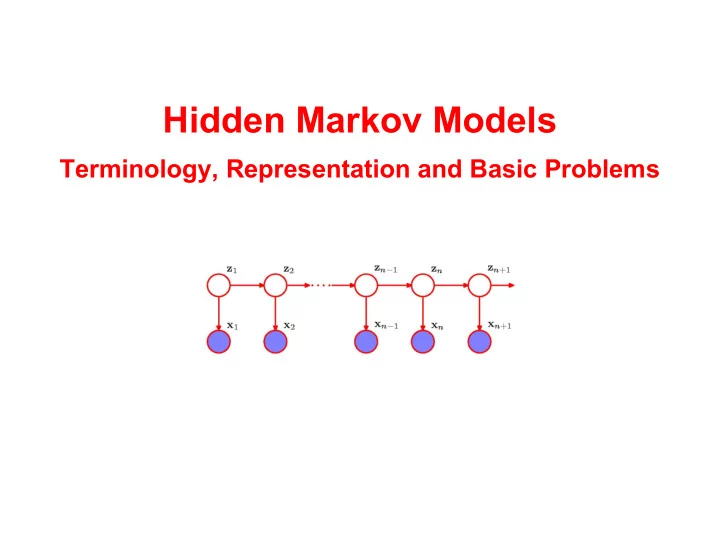
The next two weeks Hidden Markov models (HMMs): Wed 20/11: Terminology and basic algorithms. Fri 22/11: Implementing the basic algorithms. Wed 27/11: Implementing the basic algorithms, cont. Selecting model parameters and training. Fri 29/11: Selecting model parameters and training, cont. Extensions and applications. We use Chapter 13 from Bishop's book “Pattern Recognition and Machine Learning”. Rabiner's paper “A Tutorial on Hidden Markov Models [...]” might also be useful to read. Blackboard and http://birc.au.dk/~cstorm/courses/ML_e19

What is machine learning? Machine learning means different things to different people, and there is no general agreed upon core set of algorithms that must be learned. For me, the core of machine learning is: Building a mathematical model that captures some desired structure of the data that you are working on. Training the model (i.e. set the parameters of the model) based on existing data to optimize it as well as we can. Making predictions by using the model on new data.

Data – Observations A sequence of observations from a finite and discrete set, e.g. measurements of weather patterns, daily values of stocks, the composition of DNA or proteins, or ... Typical question/problem: How likely is a given X , i.e. p( X )? We need a model that describes how to compute p( X )

Simple Models (1) Observations are independent and identically distributed Too simplistic for realistic modelling of many phenomena

Simple Models (2) The n' th observation in a chain of observations is influenced only by the n -1'th observation, i.e. The chain of observations is a 1st-order Markov chain, and the probability of a sequence of N observations is

The model, i.e. p ( x n | x n -1 ): A sequence of observations: Simple Models (2) The n' th observation in a chain of observations is influenced only by the n -1'th observation, i.e. The chain of observations is a 1st-order Markov chain, and the probability of a sequence of N observations is

Hidden Markov Models What if the n' th observation in a chain of observations is influenced by a corresponding hidden variable? Latent values H H L L H Observations If the hidden variables are discrete and form a Markov chain, then it is a hidden Markov model (HMM)

Hidden Markov Models What if the n' th observation in a chain of observations is influenced by a corresponding hidden variable? Latent values Markov Model H H L L H Hidden Markov Model Observations If the hidden variables are discrete and form a Markov chain, then it is a hidden Markov model (HMM)

Hidden Markov Models What if the n' th observation in a chain of observations is influenced The joint distribution by a corresponding hidden variable? Latent values Markov Model H H L L H Hidden Markov Model Observations If the hidden variables are discrete and form a Markov chain, then it is a hidden Markov model (HMM)

Hidden Markov Models Emission probabilities What if the n' th observation in a chain of observations is influenced Transition probabilities The joint distribution by a corresponding hidden variable? Latent values Markov Model H H L L H Hidden Markov Model Observations If the hidden variables are discrete and form a Markov chain, then it is a hidden Markov model (HMM)

Transition probabilities Notation: In Bishop, the hidden variables z n are positional vectors, e.g. if z n = (0,0,1) then the model in step n is in state k =3 Transition probabilities: If the hidden variables are discrete with K states, the conditional distribution p ( z n | z n -1 ) is a K x K table A , and the marginal distribution p ( z 1 ) describing the initial state is a K vector π The probability of going from The probability of state k state j to state k is: being the initial state is:

Transition probabilities Notation: In Bishop, the hidden variables z n are positional vectors, e.g. if z n = (0,0,1) then the model in step n is in state k =3 ... Transition probabilities: If the hidden variables are discrete with K states, the conditional distribution p ( z n | z n -1 ) is a K x K table A , and the marginal distribution p ( z 1 ) describing the initial state is a K vector π ... The probability of going from The probability of state k state j to state k is: being the initial state is:

Transition Probabilities The transition probabilities: Notation: In Bishop, the hidden variables z n are positional vectors, e.g. if z n = (0,0,1) then the model in step n is in state k =3 ... Transition probabilities: If the hidden variables are discrete with K states, the conditional distribution p ( z n | z n -1 ) is a K x K table A , and the marginal distribution p ( z 1 ) describing the initial state is a K vector π ... The probability of going from The probability of state k state j to state k is: being the initial state is:

Emission probabilities Emission probabilities: The conditional distributions of the observed variables p ( x n | z n ) from a specific state If the observed values x n are discrete (e.g. D symbols), the emission probabilities Ф is a K x D table of probabilities which for each of the K states specifies the probability of emitting each observable ...

Emission probabilities Emission probabilities: The conditional distributions of the observed variables p ( x n | z n ) from a specific state If the observed values x n are discrete (e.g. D symbols), the emission probabilities Ф is a K x D table of probabilities which for each of the K states specifies the probability of emitting each observable ...

HMM joint probability distribution Observables: Latent states: Model parameters: If A and Ф are the same for all n then the HMM is homogeneous

Example – 2-state HMM Observable: {A, C, G, T}, States: {0,1} 0.95 0.05 0.25 0.25 0.25 0.25 π φ 1.00 A 0.10 0.90 0.20 0.30 0.30 0.20 0.00 0.10 0.05 A: 0.25 A: 0.15 C: 0.25 C: 0.30 G: 0.25 G: 0.20 T: 0.25 T: 0.35 0 1 0.95 0.90

Example – 7-state HMM Observable: {A, C, G, T}, States: {0,1, 2, 3, 4, 5, 6} 0.00 0.00 0.90 0.10 0.00 0.00 0.00 0.30 0.25 0.25 0.20 0.00 1.00 0.00 0.00 0.00 0.00 0.00 0.00 0.20 0.35 0.15 0.30 0.00 0.00 1.00 0.00 0.00 0.00 0.00 0.00 0.40 0.15 0.20 0.25 0.00 0.00 0.00 0.05 0.90 0.05 0.00 0.00 0.25 0.25 0.25 0.25 1.00 0.00 0.00 0.00 0.00 0.00 1.00 0.00 0.20 0.40 0.30 0.10 0.00 0.00 0.00 0.00 0.00 0.00 0.00 1.00 0.30 0.20 0.30 0.20 0.00 A π φ 0.00 0.00 0.00 0.10 0.90 0.00 0.00 0.15 0.30 0.20 0.35 0.00 0.10 0.10 0.90 0.90 0.05 0.05 A: 0.30 A: 0.20 A: 0.40 A: 0.25 A: 0.20 A: 0.30 A: 0.15 1 1 1 1 C: 0.25 C: 0.35 C: 0.15 C: 0.25 C: 0.40 C: 0.20 C: 0.30 G: 0.25 G: 0.15 G: 0.20 G: 0.25 G: 0.30 G: 0.30 G: 0.20 T: 0.20 T: 0.30 T: 0.25 T: 0.25 T: 0.10 T: 0.20 T: 0.35 0 1 2 3 4 5 6 0.90

HMMs as a generative model A HMM generates a sequence of observables by moving from latent state to latent state according to the transition probabilities and emitting an observable (from a discrete set of observables, i.e. a finite alphabet) from each latent state visited according to the emission probabilities of the state ... Model M : A run follows a sequence of states: H H L L H And emits a sequence of symbols:

Computing P(X,Z) def joint_prob(x, z): """ Returns the joint probability of x and z """ p = init_prob[z[0]] * emit_prob[z[0]][x[0]] for i in range(1, len(x)): p = p * trans_prob[z[i-1]][z[i]] * emit_prob[z[i]][x[i]] return p

Computing P(X,Z) $ python hmm_jointprob.py hmm-7-state.txt test_seq100.txt > seq100 p(x,z) = 1.8619524290102162e-65 def joint_prob(x, z): $ python hmm_jointprob.py hmm-7-state.txt test_seq200.txt > seq200 """ p(x,z) = 1.6175774997005771e-122 Returns the joint probability of x and z $ python hmm_jointprob.py hmm-7-state.txt test_seq300.txt """ > seq300 p = init_prob[z[0]] * emit_prob[z[0]][x[0]] p(x,z) = 3.0675430597843052e-183 for i in range(1, len(x)): $ python hmm_jointprob.py hmm-7-state.txt test_seq400.txt p = p * trans_prob[z[i-1]][z[i]] * emit_prob[z[i]][x[i]] > seq400 return p p(x,z) = 4.860704144302979e-247 $ python hmm_jointprob.py hmm-7-state.txt test_seq500.txt > seq500 p(x,z) = 5.258724342206735e-306 $ python hmm_jointprob.py hmm-7-state.txt test_seq600.txt > seq600 p(x,z) = 0.0

Computing P(X,Z) $ python hmm_jointprob.py hmm-7-state.txt test_seq100.txt > seq100 p(x,z) = 1.8619524290102162e-65 def joint_prob(x, z): $ python hmm_jointprob.py hmm-7-state.txt test_seq200.txt > seq200 """ p(x,z) = 1.6175774997005771e-122 Returns the joint probability of x and z $ python hmm_jointprob.py hmm-7-state.txt test_seq300.txt """ > seq300 p = init_prob[z[0]] * emit_prob[z[0]][x[0]] p(x,z) = 3.0675430597843052e-183 for i in range(1, len(x)): $ python hmm_jointprob.py hmm-7-state.txt test_seq400.txt p = p * trans_prob[z[i-1]][z[i]] * emit_prob[z[i]][x[i]] > seq400 return p p(x,z) = 4.860704144302979e-247 $ python hmm_jointprob.py hmm-7-state.txt test_seq500.txt > seq500 p(x,z) = 5.258724342206735e-306 $ python hmm_jointprob.py hmm-7-state.txt test_seq600.txt > seq600 Should be >0 by construction of X and Z p(x,z) = 0.0