Lecture 2: Exercises Frank den Hollander Elena Pulvirenti June 25, - PDF document

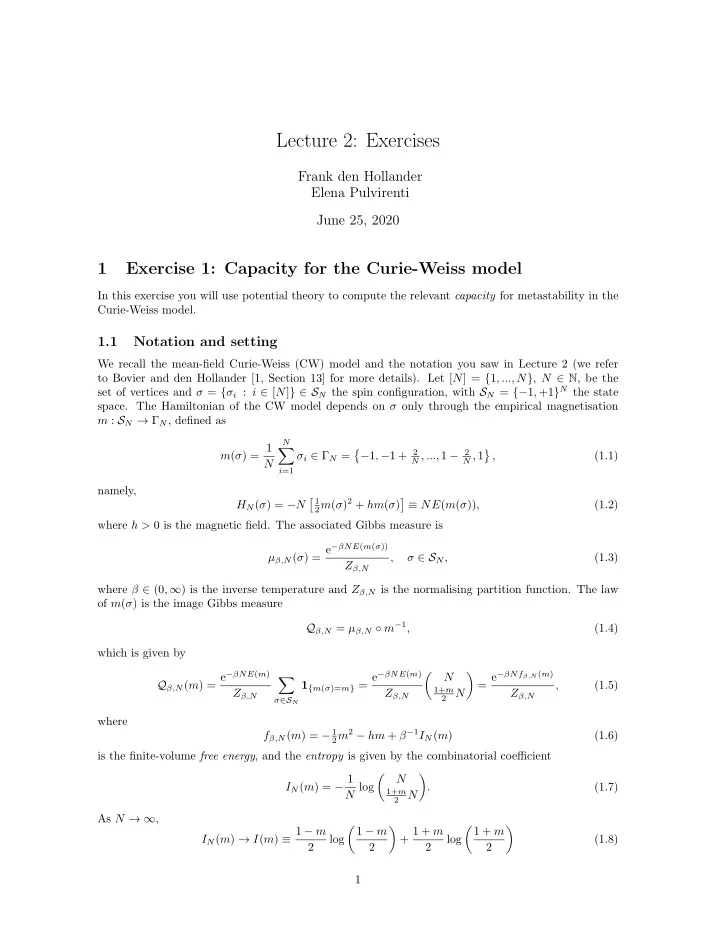
Lecture 2: Exercises Frank den Hollander Elena Pulvirenti June 25, 2020 1 Exercise 1: Capacity for the Curie-Weiss model In this exercise you will use potential theory to compute the relevant capacity for metastability in the Curie-Weiss model. 1.1 Notation and setting We recall the mean-field Curie-Weiss (CW) model and the notation you saw in Lecture 2 (we refer to Bovier and den Hollander [1, Section 13] for more details). Let [ N ] = { 1 , ..., N } , N ∈ N , be the set of vertices and σ = { σ i : i ∈ [ N ] } ∈ S N the spin configuration, with S N = {− 1 , +1 } N the state space. The Hamiltonian of the CW model depends on σ only through the empirical magnetisation m : S N → Γ N , defined as N m ( σ ) = 1 � � − 1 , − 1 + 2 N , ..., 1 − 2 � σ i ∈ Γ N = N , 1 (1.1) , N i =1 namely, � 1 2 m ( σ ) 2 + hm ( σ ) � H N ( σ ) = − N ≡ NE ( m ( σ )) , (1.2) where h > 0 is the magnetic field. The associated Gibbs measure is µ β,N ( σ ) = e − βNE ( m ( σ )) , σ ∈ S N , (1.3) Z β,N where β ∈ (0 , ∞ ) is the inverse temperature and Z β,N is the normalising partition function. The law of m ( σ ) is the image Gibbs measure Q β,N = µ β,N ◦ m − 1 , (1.4) which is given by Q β,N ( m ) = e − βNE ( m ) 1 { m ( σ )= m } = e − βNE ( m ) = e − βNf β,N ( m ) � � N � (1.5) , 1+ m Z β,N Z β,N 2 N Z β,N σ ∈S N where 2 m 2 − hm + β − 1 I N ( m ) f β,N ( m ) = − 1 (1.6) is the finite-volume free energy , and the entropy is given by the combinatorial coefficient I N ( m ) = − 1 � � N N log . (1.7) 1+ m 2 N As N → ∞ , � 1 − m � � 1 + m � I N ( m ) → I ( m ) ≡ 1 − m + 1 + m log log (1.8) 2 2 2 2 1

(which differs by a constant − log 2 from the formula in the slides) and 2 m 2 − hm + β − 1 I ( m ) . f β,N ( m ) → f β ( m ) ≡ − 1 (1.9) In fact, � 1 � 1 − m 2 � � 1 + log N + log(2 π ) I N ( m ) − I ( m ) = 2 N log + O (1.10) . 4 2 N N 2 We consider the discrete-time Markov chain { σ ( t ) } t ≥ 0 given by the Glauber dynamics on S N with Metropolis transition probabilities:  N exp( − β [ H N ( σ ′ ) − H N ( σ )] + ) , 1 if σ ∼ σ ′ ,   p N ( σ, σ ′ ) = if σ = σ ′ , 1 − � (1.11) η � = σ p ( σ, η ) ,  0 , else,  where σ ∼ σ ′ means that � σ − σ ′ � = 2 with � · � the ℓ 1 -norm on S N . A particular feature of this dynamics is that the image m ( t ) ≡ m ( σ ( t )) of σ ( t ) under the map m again is a Markov process on Γ N , with transition probabilities � if m ′ = m + 2 exp( − βN [ E ( m ′ ) − E ( m )] + ) (1 − m ) , N , r N ( m, m ′ ) = 2 (1.12) if m ′ = m − 2 exp( − βN [ E ( m ′ ) − E ( m )] + ) (1+ m ) , N . 2 This mapping is called lumping in the theory of Markov chains, see e.g. Bovier and den Hollander [1, Section 9.3]. The equilibrium CW model displays a phase transition . Namely, there is a critical value of the inverse temperature β c = 1 such that, in the regime where β > β c and h > 0 is small, the free energy f β ( m ) is a double-well function with local minimisers m − , m + and saddle point m ∗ . These are the solutions of the equation m = tanh[ β ( m + h )] . (1.13) Let m − ( N ) , m ∗ ( N ) , m + ( N ) be the points in Γ N closest to m − , m ∗ , m + respectively. Then the pair ( m − ( N ) , m + ( N )) forms a metastable set (see the slides of Lecture 2). 1.2 One-dimensional nearest-neighbour random walks Consider a Markov process with state space S ⊆ Z for which transitions are allowed between nearest- neighbour sites only. We denote the transition rates by p ( x, y ) , y = x ± 1, and denote by µ the strictly positive reversible invariant measure: µ ( x ) p ( x, y ) = µ ( y ) p ( y, x ). We state the following well-known result in the form of a lemma (see e.g. Bovier and den Hollander [1, Section 7.1.4] for more details). Lemma 1.1. For every a, b ∈ S with a < b , � − 1 � b 1 1 � cap( a, b ) = . (1.14) µ ( y ) p ( y, y − 1) y = a +1 1.3 Exercise (i) For m ∈ Γ N , the set of configurations with magnetisation m is denoted by S N [ m ]. Prove that the capacity for the Curie-Weiss model has the following asymptotics as N → ∞ : � β ( − f ′′ β ( m ∗ )) � 1 + m ∗ 1 e − βNf β ( m ∗ ) cap CW � � S N [ m − ( N )] , S N [ m + ( N )] = 1 − m ∗ [1 + o (1)] . Z β,N πN (1.15) 2

(ii) Find the following expression for the harmonic sum � − 1 � � � Q β,N ( m ) h m − ( N ) ,m + ( N ) ( m ) = e − βN f β ( m − ) (1 − m 2 − ) βf ′′ Z β,N β ( m − ) [1 + o (1)] m ∈ Γ N (1.16) 1.4 Guidelines for solving the exercise • Step 1: Start from the variational representation for the capacity (see the slides of the Intro- duction) by writing out the Dirichlet principle, i.e., � cap CW � µ β,N ( σ ) p N ( σ, σ ′ ) [ φ ( σ ) − φ ( σ ′ )] 2 , � S N [ m − ( N )] , S N [ m + ( N )] = min (1.17) φ ∈ Φ σ,σ ′ ∈S N where � � Φ := Φ S N [ m − ( N )] , S N [ m + ( N )] = φ : S N → [0 , 1]: φ | S N [ m − ( N )] = 1 , φ | S N [ m + ( N )] = 0 . (1.18) Prove that in the space Γ N the capacity can be written as cap CW � � Q β,N ( m ) r N ( m, m ′ ) [ ψ ( m ) − ψ ( m ′ )] 2 , � S N [ m − ( N )] , S N [ m + ( N )] = min (1.19) ψ ∈ Ψ m,m ′ ∈ Γ N and identify Ψ. • Step 2: Explain why the Markov chain ( m ( t )) t ∈ N 0 is a one-dimensional nearest-neighbour ran- dom walk on Γ N that is reversible with respect to the image measure Q β,N . Use this fact and Lemma 1.1 to prove that � − 1 � cap CW ( S N [ m − ( N )] , S N [ m + ( N )]) = � F ( m ) (1.20) Z β,N , m − ≤ m<m + where F ( x ) = e βNf β,N ( x ) exp(2 β [ − 1 N − ( x + h )] + ) . (1.21) (1 − x ) 2 • Step 3: Prove the identity � � = 1 − m ∗ � − 1 � N − ( m ∗ + h ) exp 2 β 1 + m ∗ [1 + o (1)] (1.22) + for N large enough. [Hint: Use the fact that m ∗ is a solution of (1.13).] • Step 4: Multiply and divide by F ( m ∗ ) inside the parenthesis in the right-hand side of (1.20). Prove that the sum can be restricted to | m − m ∗ | ≤ ε for ε > 0 small enough such that m + h < 0. • Step 5: Prove that � 2 e − βNf β,N ( m ) = e − βNf β ( m ) πN (1 − m 2 ) [1 + o (1)] (1.23) and use this inside the sum in (1.20). • Step 6: Compute the sum by applying the Laplace method of steepest descent. Take the limit ε → 0, and use again the expansion in (1.23) to conclude the computation of the capacity. • Step 7: In order to estimate the sum in the left-hand side of (1.16), use the mean hitting time formula for the Curie–Weiss model in Lecture 2 (see slide 10) and formula (1.8) in the exercise set “Introduction: Exercises”. 3

2 Exercise 2: Flow for the Curie-Weiss model In this exercise you will find a unit flow for the Curie-Weiss model. 2.1 Notation and Thomson principle We consider the same model as in Exercise 1 and recall a key tool for the potential-theoretic approach to metastability, i.e., Thomson principle. We start with the definition of unit flow (for more background, see Bovier and den Hollander [1, Chapters 7–8]). Definition 2.1. Let G = ( V, E ) be a graph and let A, B be disjoint subsets of V . A map u : E → R is called a unit flow from A to B if it satisfies the following properties: 1. Kirchhoff’s law : The flows into and out of vertices in V \ ( A ∪ B ) are the same, i.e., � � u ( y, x ) = u ( x, w ) , ∀ x ∈ V \ ( A ∪ B ) . (2.1) y ∈ V : w ∈ V : ( x,w ) ∈ E ( y,x ) ∈ E 2. The total flow out of A and into B is 1 , i.e., � � � � u ( a, y ) = 1 = u ( y, b ) . (2.2) a ∈ A y ∈ V : b ∈ B y ∈ V : ( a,y ) ∈ E ( y,b ) ∈ E For Markov processes with countable state space S , take the graph to be ( S , E ), where the edge set is induced by the transition probabilities p ( x, y ) of the dynamics (i.e., an edge between two states is present if and only if the Markov chain has a positive probability to go from one to the other in a single step). We are now ready to recall the following formulation of the Thomson principle in terms of flows (see e.g. Bovier and den Hollander [1, Section 7.3.2]). Let U AB be the space of all unit flows from A to B as in Definition 2.1. Then the Thomson principle states that 1 cap( A, B ) = sup (2.3) D ( u ) u ∈U AB with u ( x, y ) 2 � D ( u ) = µ ( x ) p ( x, y ) , (2.4) ( x,y ) ∈ E where E is the set of pairs ( x, y ) such that p ( x, y ) � = 0 with x, y ∈ S and µ is the equilibrium measure. The supremum in (2.3) is uniquely attained at u h AB ( x, y ) = µ ( x ) p ( x, y )[ h AB ( y ) − h AB ( x )] + , (2.5) cap( A, B ) i.e., the harmonic unit flow . This variational principle is a powerful tool for asymptotic computations of capacities. In fact, by guessing a good test flow we can easily get a lower bound for the capacity. We saw in the previous exercise that the CW model is perfectly lumpable, meaning that we can compute the mean metastable crossover time by exploiting the fact that in the space of magnetisations the model behaves like a random walk. In this exercise, instead, you will see how to choose a good unit flow for the CW model. 4