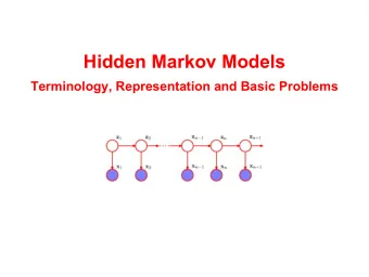
Markov Models Yanbing Xue Outline Introduction Markov chains - PDF document

2020 年 2 月 25 日 Markov Models Yanbing Xue Outline ▪ Introduction ▪ Markov chains ▪ Dynamic belief networks ▪ Hidden Markov models (HMMs) 1

2020 年 2 月 25 日 Outline ▪ Introduction ▪ Time series ▪ Probabilistic graphical models ▪ Markov chains ▪ Dynamic belief networks ▪ Hiddem Markov models (HMM) What is time series? ▪ A time series is a sequence of data instance listed in time order. ▪ In other words, data instances are totally ordered. ▪ Example: weather forecasting ▪ Notice: we care about the orderings rather than the exact time. 2

2020 年 2 月 25 日 Different kinds of time series ▪ Two properties: ▪ Time space: discrete or continuous ? ▪ Task: classification or regression ? Discrete & classification Weather Min/max temp Discrete & regression Temperature Continuous & regression Prob of rain Probabilistic graphical models (PGMs) ▪ A PGM uses a graph-based representation to represent the conditional distributions over variables. ▪ Directed acyclic graphs (DAGs) Markov model is a sub- family of PGMs on DAGs ▪ Undirected graph 3

2020 年 2 月 25 日 Outline ▪ Introduction ▪ Markov chains ▪ Intuition ▪ Inference ▪ Learning ▪ Dynamic belief networks ▪ Hidden Markov models (HMMs) Modeling time series Assume a sequence of four weather observations: 𝑧 1 , 𝑧 2 , 𝑧 3 , 𝑧 4 𝑧 1 𝑧 2 𝑧 3 𝑧 4 ▪ Possible dependences: 𝑧 4 depends on the previous weather(s) 𝑧 1 𝑧 2 𝑧 3 𝑧 4 4

2020 年 2 月 25 日 Modeling time series In general observations: 𝑧 1 , 𝑧 2 , 𝑧 3 , 𝑧 4 can be y 1 y 2 y 3 y 4 y 1 y 2 y 3 y 4 A lot of middle ground in between the two extremes Fully dependent: Independent: E.g. y 4 depends on all E.g. y 4 does not depend on previous observations any previous observation Modeling time series ▪ Are there intuitive and convenient dependency models? ? y 1 y 2 y 3 y 4 y 1 y 2 y 3 y 4 Think of the last observation 𝑄(𝑧 4 |𝑧 1 𝑧 2 𝑧 3 ) Totally drops time What if we have T observations? information Parameter #: exponential to # of observations 5

2020 年 2 月 25 日 Markov chains ▪ Markov assumption : Future predictions are independent of all but the most recent observations y 1 y 2 y 3 y 4 y 1 y 2 y 3 y 4 y 1 y 2 y 3 y 4 First order Markov chain Fully dependent Independent Markov chains ▪ Markov assumption : Future predictions are independent of all but the most recent observations y 1 y 2 y 3 y 4 y 1 y 2 y 3 y 4 y 1 y 2 y 3 y 4 Fully dependent Independent Second order Markov chain 6

2020 年 2 月 25 日 A formal representation ▪ Using conditional probabilities to model 𝑧 1 , 𝑧 2 , 𝑧 3 , 𝑧 4 ▪ Fully dependent: ▪ 𝑄 𝑧 1 𝑧 2 𝑧 3 𝑧 4 = 𝑄 𝑧 1 𝑄 𝑧 2 𝑧 1 𝑄 𝑧 3 𝑧 1 𝑧 2 𝑄(𝑧 4 |𝑧 1 𝑧 2 𝑧 3 ) ▪ Fully independent: ▪ 𝑄 𝑧 1 𝑧 2 𝑧 3 𝑧 4 = 𝑄 𝑧 1 𝑄(𝑧 2 )𝑄(𝑧 3 )𝑄(𝑧 4 ) ▪ First-order Markov chain (recent 1 observation): ▪ 𝑄 𝑧 1 𝑧 2 𝑧 3 𝑧 4 = 𝑄 𝑧 1 𝑄 𝑧 2 𝑧 1 𝑄 𝑧 3 𝑧 2 𝑄(𝑧 4 |𝑧 3 ) ▪ Second-order Markov chain (recent 2 observations): ▪ 𝑄 𝑧 1 𝑧 2 𝑧 3 𝑧 4 = 𝑄 𝑧 1 𝑄 𝑧 2 𝑧 1 𝑄 𝑧 3 𝑧 1 𝑧 2 𝑄(𝑧 4 |𝑧 2 𝑧 3 ) A more formal representation ▪ Generalizes to T observations ▪ First-order Markov chain (recent 1 observation): ▪ 𝑄 𝑧 1 𝑧 2 … 𝑧 𝑈 = 𝑄 𝑧 1 ς 𝑢=2 𝑈 𝑄(𝑧 𝑢 |𝑧 𝑢−1 ) ▪ Second-order Markov chain (recent 2 observations): ▪ 𝑄 𝑧 1 𝑧 2 … 𝑧 𝑈 = 𝑄 𝑧 1 𝑄 𝑧 2 𝑧 1 ς 𝑢=3 𝑈 𝑄(𝑧 𝑢 |𝑧 𝑢−1 𝑧 𝑢−2 ) ▪ k-th order Markov chain (recent k observations): 𝑈 ▪ 𝑄 𝑧 1 𝑧 2 … 𝑧 𝑈 = 𝑄 𝑧 1 𝑄 𝑧 2 𝑧 1 … 𝑄(𝑧 𝑙 |𝑧 1 … 𝑧 𝑙−1 )ς 𝑢=𝑙+1 𝑄(𝑧 𝑢 |𝑧 𝑢−𝑙 … 𝑧 𝑢−1 ) 7

2020 年 2 月 25 日 Stationarity ▪ Do all states yield to the identical conditional distribution? ▪ 𝑄 𝑧 𝑢 = 𝑘 𝑧 𝑢−1 = 𝑗 = 𝑄 𝑧 𝑢−1 = 𝑘 𝑧 𝑢−2 = 𝑗 for all 𝑢, 𝑗, 𝑘 ▪ Typically holds 𝐵 11 ⋯ 𝐵 1𝑒 ▪ A transition table A to represent conditional distribution ⋮ ⋱ ⋮ 𝐵 𝑒1 ⋯ 𝐵 𝑒𝑒 ▪ 𝐵 𝑗𝑘 = 𝑄 𝑧 𝑢 = 𝑘 𝑧 𝑢−1 = 𝑗 for all 𝑢 = 1,2, … , 𝑈 ▪ 𝑒 : dimention of 𝑧 𝑢 ▪ A vector 𝛒 to represent the initial distribution ▪ 𝜌 𝑗 = 𝑄(𝑧 1 = 𝑗) for all 𝑗 = 1,2, … , 𝑒 Inference on a Markov chain ▪ Probability of a given sequence 𝑈 ▪ 𝑄 𝑧 1 = 𝑗 1 , … , 𝑧 𝑈 = 𝑗 𝑈 = 𝜌 𝑗 1 ς 𝑢=2 𝐵 𝑗 𝑢 𝑗 𝑢−1 ▪ Probability of a given state ▪ Forward iteration: 𝑄 𝑧 𝑢 = 𝑗 𝑢 = σ 𝑗 𝑢−1 𝑄(𝑧 𝑢−1 = 𝑗 𝑢−1 )𝐵 𝑗 𝑢 𝑗 𝑢−1 ▪ Can be calculated iteratively ▪ Both inferences are efficient 𝑈 ▪ 𝑄 𝑧 𝑙 = 𝑗 𝑙 , … , 𝑧 𝑈 = 𝑗 𝑈 = 𝑄 𝑧 𝑙 = 𝑗 𝑙 ς 𝑢=𝑙+1 𝐵 𝑗 𝑢 𝑗 𝑢−1 8

2020 年 2 月 25 日 Learning a Markov chain ▪ MLE of conditional probabilities can be estimated directly. 𝑁𝑀𝐹 = 𝑄 𝑧 𝑢 = 𝑘 𝑧 𝑢−1 = 𝑗 = 𝑄(𝑧 𝑢 =𝑘,𝑧 𝑢−1 =𝑗) 𝑂 𝑗𝑘 ▪ 𝐵 𝑗𝑘 = σ 𝑘 𝑂 𝑗𝑘 𝑄(𝑧 𝑢−1 =𝑗) ▪ 𝑂 𝑗𝑘 : # of observations that yields 𝑧 𝑢 = 𝑘, 𝑧 𝑢−1 = 𝑗 ▪ Bayesian parameter estimation ▪ Prior: 𝐸𝑗𝑠(𝜄 1 , 𝜄 2 , … ) ▪ Posterior: 𝐸𝑗𝑠(𝜄 1 + 𝑂 𝑗1 , 𝜄 2 + 𝑂 𝑗2 , … ) 𝑁𝐵𝑄 = 𝑂 𝑗𝑘 +𝜄 𝑘 −1 𝐹𝑊 = 𝑂 𝑗𝑘 +𝜄 𝑘 ▪ 𝐵 𝑗𝑘 𝐵 𝑗𝑘 σ 𝑘 (𝑂 𝑗𝑘 +𝜄 𝑘 −1) σ 𝑘 (𝑂 𝑗𝑘 +𝜄 𝑘 ) A toy example – weather forecast ▪ State 1: rainy state 2: cloudy state 3: sunny ▪ Given “sun -sun-sun-rain-rain-sun-cloud- sun”, find 𝐵 33 𝑁𝑀𝐹 = 𝑂 33 2 ▪ 𝐵 33 σ 𝑘 𝑂 3𝑘 = 1+1+2 ▪ Prior: 𝐸𝑗𝑠(2,2,2) ▪ Posterior: 𝐸𝑗𝑠(2 + 1,2 + 1,2 + 2) 𝑁𝐵𝑄 = 𝑂 33 +𝜄 3 −1 3 𝐹𝑊 = 𝑂 33 +𝜄 3 4 ▪ 𝐵 33 σ 𝑘 (𝑂 3𝑘 +𝜄 𝑘 −1) = 𝐵 33 σ 𝑘 (𝑂 3𝑘 +𝜄 𝑘 ) = 7 10 9

2020 年 2 月 25 日 A toy example – weather forecast 0.4 0.3 0.3 ▪ Given 𝐵 = 0.2 0.6 0.2 , day 1 is sunny 0.1 0.1 0.8 ▪ Find the probability that day 2~8 will be “sun -sun-rain-rain-sun-cloud- sun” ▪ 𝑄 𝑧 1 𝑧 2 … 𝑧 8 = 𝑄 𝑧 1 = 𝑡 𝑄 𝑧 2 = 𝑡 𝑧 1 = 𝑡 𝑄 𝑧 3 = 𝑡 𝑧 2 = 𝑡 𝑄 𝑧 4 = 𝑠 𝑧 3 = 𝑡 𝑄 𝑧 5 = 𝑠 𝑧 4 = 𝑠 𝑄 𝑧 6 = 𝑡 𝑧 5 = 𝑠 𝑄 𝑧 7 = 𝑑 𝑧 6 = 𝑡 𝑄 𝑧 8 = 𝑡 𝑧 7 = 𝑑 = 1 ∙ 𝐵 33 ∙ 𝐵 33 ∙ 𝐵 31 ∙ 𝐵 11 ∙ 𝐵 13 ∙ 𝐵 32 ∙ 𝐵 23 = 1 ∙ 0.8 ∙ 0.8 ∙ 0.1 ∙ 0.4 ∙ 0.3 ∙ 0.1 ∙ 0.2 = 1.536 × 10 −4 A toy example – weather forecast 0.4 0.3 0.3 ▪ Given 𝐵 = 0.2 0.6 0.2 , day 1 is sunny 0.1 0.1 0.8 ▪ Find the probability that day 3 will be sunny ▪ 𝑄 𝑧 2 = 𝑡 = σ 𝑗 𝑄 𝑧 1 = 𝑗 𝑄 𝑧 2 = 𝑡 𝑧 1 = 𝑗 = 0 ∙ 0.3 + 0 ∙ 0.2 + 1 ∙ 0.8 = 0.8 ▪ Similarly, 𝑄 𝑧 2 = 𝑠 = σ 𝑗 𝑄 𝑧 1 = 𝑗 𝑄 𝑧 2 = 𝑠 𝑧 1 = 𝑗 = 0 ∙ 0.4 + 0 ∙ 0.2 + 1 ∙ 0.1 = 0.1 ▪ 𝑄 𝑧 2 = 𝑑 = σ 𝑗 𝑄 𝑧 1 = 𝑗 𝑄 𝑧 2 = 𝑑 𝑧 1 = 𝑗 = 0 ∙ 0.3 + 0 ∙ 0.6 + 1 ∙ 0.1 = 0.1 ▪ 𝑄 𝑧 3 = 𝑡 = σ 𝑗 𝑄 𝑧 2 = 𝑗 𝑄 𝑧 3 = 𝑡 𝑧 2 = 𝑗 = 0.1 ∙ 0.3 + 0.1 ∙ 0.2 + 0.8 ∙ 0.8 = 0.69 10

2020 年 2 月 25 日 Limitation of Markov chain ▪ Each state is represented by one variable ▪ What if each state consists of multiple variables? Outline ▪ Introduction ▪ Markov chains ▪ Dynamic belief networks ▪ Intuition ▪ Inference ▪ Learning ▪ Hidden Markov models (HMMs) 11

2020 年 2 月 25 日 Modeling multiple variables ▪ What if each state consists of multiple variables? ▪ e.g. monitoring a robot ▪ Location, GPS, Speed L t-1 G t-1 S t-1 L t G t S t ▪ Modeling all variables in each state jointly ▪ Is this a good solution? Modeling multiple variables L t-1 G t-1 S t-1 L t G t S t ▪ Each variable only depends on some of the previous or current observations ▪ Factorization S t-1 S t L t-1 L t G t-1 G t 12

2020 年 2 月 25 日 Dynamic belief networks ▪ Also named as dynamic Bayesian networks 𝐘 𝑢 = {𝑇 𝑢 , 𝑀 𝑢 } : transition states S t-1 S t Only dependent on previous observations L t-1 L t 𝑄 𝐘 𝑢 𝐘 𝑢−1 = {𝑄 𝑇 𝑢 𝑇 𝑢−1 , 𝑄 𝑀 𝑢 𝑇 𝑢−1 𝑀 𝑢−1 } : 𝐙 𝑢 = {𝐻 𝑢 } : emission states / evidences transition model Only dependent on current G t-1 G t observations 𝑄 𝐙 𝑢 𝐘 𝑢 = {𝑄 𝐻 𝑢 𝑀 𝑢 } : emission model / sensor model Inference on a dynamic BN ▪ Filtering: given 𝐳 1…𝑢 , find 𝑄(𝐘 𝑢 |𝐳 1…𝑢 ) ▪ Exact inference ▪ using Bayesian rule and the structure of dynamic BN ▪ 𝑄 𝐘 𝑢 𝐳 1…𝑢 Can be inferred iteratively ∝ 𝑄 𝐘 𝑢 𝐳 𝑢 𝐳 1…𝑢−1 = 𝑄 𝐳 𝑢 𝐘 𝑢 𝐳 1…𝑢−1 𝑄 𝐘 𝑢 𝐳 1…𝑢−1 Structure of dynamic BN = 𝑄 𝐳 𝑢 𝐘 𝑢 𝐳 1…𝑢−1 ෍ 𝑄 𝐘 𝑢 𝐲 𝑢−1 𝐳 1…𝑢−1 𝑄 𝐲 𝑢−1 𝐳 1…𝑢−1 𝐲 𝑢−1 Emission model Transition model 13