Math 283, Spring 2006, Prof. Tesler May 22, 2006 Markov chains and - PDF document

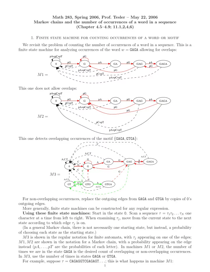
Math 283, Spring 2006, Prof. Tesler – May 22, 2006 Markov chains and the number of occurrences of a word in a sequence (Chapter 4.5–4.9; 11.1,2,4,6) 1. Finite state machine for counting occurrences of a word or motif We revisit the problem of counting the number of occurrences of a word in a sequence. This is a finite state machine for analyzing occurrences of the word w = GAGA allowing for overlaps: pA+pC+pT pG pG pA pG pA 0 G GA GAG GAGA pC+pT pG pA+pC+pT pG pC+pT M 1 = pA+pC+pT This one does not allow overlaps: pA+pC+pT pG pG pA pG pA 0 G GA GAG GAGA pC+pT pA+pC+pT pG pG M 2 = pC+pT pA+pC+pT This one detects overlapping occurrences of the motif { GAGA , GTGA } : C A,C,T A,C,T A,C,T G G A C GA GAG GAGA A G G 0 G G T C T G M 3 = A,C,T G T G A GT GTG GTGA A,C,T For non-overlapping occurrences, replace the outgoing edges from GAGA and GTGA by copies of 0 ’s outgoing edges. More generally, finite state machines can be constructed for any regular expression. Using these finite state machines: Start in the state 0 . Scan a sequence τ = τ 1 τ 2 . . . τ N one character at a time from left to right. When examining τ j , move from the current state to the next state according to which edge τ j is on. (In a general Markov chain, there is not necessarily one starting state, but instead, a probability of choosing each state as the starting state.) M 3 is shown in the regular notation for finite automata, with τ j appearing on one of the edges; M 1 , M 2 are shown in the notation for a Markov chain, with a probability appearing on the edge instead ( pA, . . . , pT are the probabilities of each letter). In machines M 1 or M 2, the number of times we are in the state GAGA is the desired count of overlapping or non-overlapping occurrences. In M 3, use the number of times in states GAGA or GTGA . For example, suppose τ = CAGAGGTCGAGAGT... ; this is what happens in machine M 1: 1

2 Time t State at t τ t +1 Time t State at t τ t +1 Time t State at t τ t +1 1 6 11 0 C GAG G GA G 2 7 12 0 A G T GAG A 3 0 G 8 0 C 13 GAGA G 4 9 14 G A 0 G GAG T · · · 5 GA G 10 G A 15 0 In machine M 2, the only difference is that t = 14 is state G . Names of states in overlapping case ( M 1 ): If we are in state w 1 . . . w r after examining τ j , it means that the last r letters of τ ending at τ j agreed with the first r letters of w , and that there is not a longer prefix of w that ends at τ j . Names of states in non-overlapping case ( M 2 ): It’s almost the same as M 1, except the outgoing edges of GAGA are replaced by copies of the outgoing edges of 0 (same probabilities and endpoints but starting at GAGA instead of starting at 0 ), so that the second GA cannot count towards an overlapping occurrence of GAGA . Names of states in motif, overlapping case ( M 3 ): State w 1 . . . w r means the last r letters of τ ending at τ j are w 1 . . . w r ; some word in the motif starts with w 1 . . . w r ; and there isn’t a longer word ending at τ j that is a prefix of any word in the motif. This is how to design a machine like M 1 for any word (to analyze overlapping occurrences of the word w = w 1 w 2 . . . w k ): (a) Make a graph with k + 1 nodes (called “states”): ∅ , w 1 , w 1 w 2 , w 1 w 2 w 3 , . . . , w 1 w 2 · · · w k . (b) Each node has four outgoing edges (which may later be merged into fewer). For each node w 1 . . . w r and each letter x = A , C , G , T , determine the longest suffix s (possibly ∅ ) of w 1 . . . w r x that is one of the states. Draw an edge from w 1 . . . w r to s , with probability p x on that edge. Note that if r < k and x = w r +1 , this will be an edge to w 1 . . . w r +1 . (c) If there are several edges in the same direction between two nodes, combine them into one edge by adding the probabilities together. For non-overlapping occurrences of w (as in M 2), replace the outgoing edges from w by copies of 0 ’s outgoing edges. For motifs (overlapping or non-overlapping), the states are all the prefixes of all the words. If a prefix is common to more than one word, it is only used as one state. 2. Markov chains A Markov chain is similar to a finite state machine, but incorporates probabilities. Let S be a set of “states.” We will take S to be a discrete finite set, such as S = { 1 , 2 , . . . , s } . Let t = 1 , 2 , . . . denote the “time.” Let X 1 , X 2 , . . . denote a sequence of random variables, which take on values from S . The X t ’s form a Markov chain if they obey these rules: (1) The probability of being in a certain state at time t + 1 only depends on the state at time t , not on any earlier states: P ( X t +1 = x t +1 | X 0 = x 0 , . . . , X t = x t ) = P ( X t +1 = x t +1 | X t = x t ): (2) The probability of transitioning from state i at time t to state j at time t + 1 only depends on i and j , and does not depend on the time: there are values p ij such that P ( X t +1 = j | X t = i ) = p ij at all times t . These are put into an s × s transition matrix . The transition matrix , P 1, of the Markov chain M 1 is

3 To state 1 2 3 4 5     From state 1: 0 p A + p C + p T p G 0 0 0 P 11 P 12 P 13 P 14 P 15     From state 2: G p C + p T p G p A 0 0 P 21 P 22 P 23 P 24 P 25         From state 3: GA p A + p C + p T 0 0 p G 0 = P 31 P 32 P 33 P 34 P 35         From state 4: GAG p C + p T p G 0 0 p A P 41 P 42 P 43 P 44 P 45 From state 5: GAGA p A + p C + p T 0 0 p G 0 P 51 P 52 P 53 P 54 P 55 Notice that the entries in each row sum up to p A + p C + p G + p T = 1. A matrix with all entries ≥ 0 and all row sums equal to 1 is called a stochastic matrix . The transition matrix of a Markov chain is always a stochastic matrix. (For state machines in other contexts than Markov Chains, the transition matrix would have weights = 0 for no edge or � = 0 for an edge, but the nonzero weights may be defined differently, and the matrices are usually not stochastic.) For M 2, since edges leaving GAGA were changed to copy 0 ’s outgoing edges, the bottom row changes to a copy of the top row. If all nucleotides have equal probabilities p A = p C = p G = p T = 1 4 , matrices P 1 and P 2 become     3 / 4 1 / 4 0 0 0 3 / 4 1 / 4 0 0 0     1 / 2 1 / 4 1 / 4 0 0 1 / 2 1 / 4 1 / 4 0 0         P 1 = 3 / 4 0 0 1 / 4 0 P 2 = 3 / 4 0 0 1 / 4 0         1 / 2 1 / 4 0 0 1 / 4 1 / 2 1 / 4 0 0 1 / 4 3 / 4 0 0 1 / 4 0 3 / 4 1 / 4 0 0 0 We will examine several questions that apply to Markov chains, using P 1 or P 2 as examples. (1) What is the probability of being in a particular state after n steps? (2) What is the probability of being in a particular state as n → ∞ ? (3) What is the “reverse” Markov chain? (4) If you are in state i , what is the expected number of time steps until the next time you are in state j ? What is the variance of this? What is the complete probability distribution? (5) Starting in state i , what is the expected number of visits to state j before reaching state k ? 2.1. Technical conditions. This Markov chain has a number of complications: 1 2 4 7 8 9 M 4 = 3 5 6 10 A Markov chain is irreducible if every state can be reached from every other state after enough steps. But M 4 is reducible since there are states that cannot be reached from each other: after sufficient time, you are either stuck in state 3, the component { 4 , 5 , 6 , 7 } , or the component { 8 , 9 , 10 } . State i has period d if the Markov chain can only go from state i to itself in multiples of d steps, where d is the maximum number that satisfies that. If d > 1 then state i is periodic. A Markov chain is periodic if at least one state is periodic and is aperiodic if no states are periodic. All states in a component have the same period. In M 4, component { 4 , 5 , 6 , 7 } has period 2 and component { 8 , 9 , 10 } has period 3, so M 4 is periodic. An absorbing state has all its outgoing edges going to itself. An irreducible Markov chain with two or more states cannot have any absorbing states. In M 4, state 3 is an absorbing state. There are generalizations to infinite numbers of discrete or continuous states and to continuous time, which we do not consider. We will work with Markov chains that are finite, discrete, irre- ducible, and aperiodic, unless otherwise stated. For a finite discrete Markov chain on two or more states, being irreducible and aperiodic with no absorbing states is equivalent to P or a power of P having all entries be greater than 0.