Example MDP 3 + 1 Complex decisions 2 1 0.8 0.1 0.1 1 - PDF document

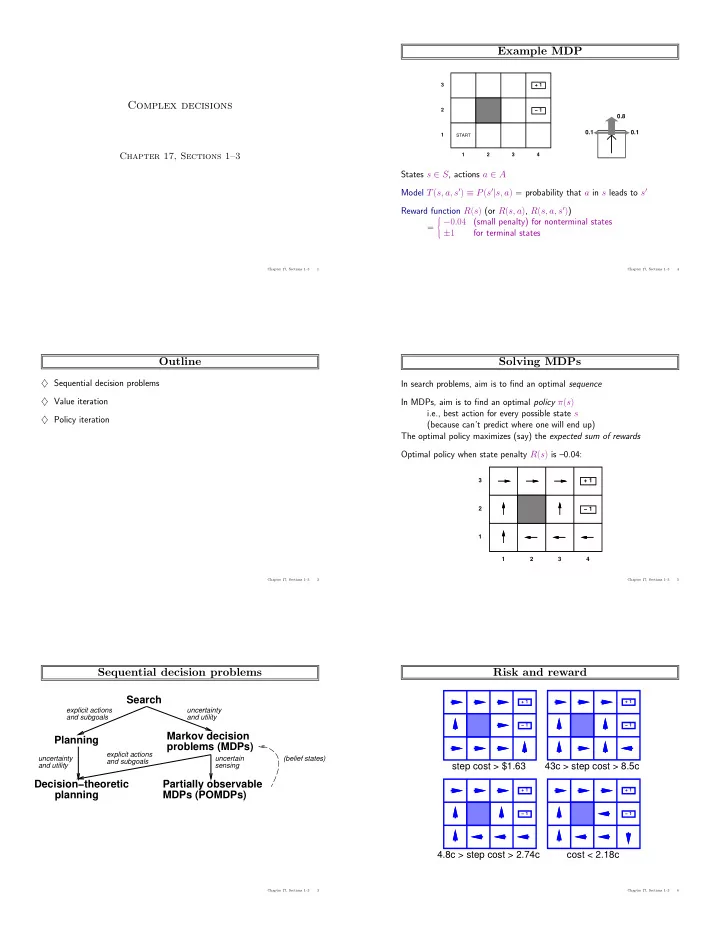
Example MDP 3 + 1 Complex decisions 2 − 1 0.8 0.1 0.1 1 START 1 2 3 4 Chapter 17, Sections 1–3 States s ∈ S , actions a ∈ A Model T ( s, a, s ′ ) ≡ P ( s ′ | s, a ) = probability that a in s leads to s ′ Reward function R ( s ) (or R ( s, a ) , R ( s, a, s ′ ) )  − 0 . 04 (small penalty) for nonterminal states  =   ± 1 for terminal states    Chapter 17, Sections 1–3 1 Chapter 17, Sections 1–3 4 Outline Solving MDPs ♦ Sequential decision problems In search problems, aim is to find an optimal sequence ♦ Value iteration In MDPs, aim is to find an optimal policy π ( s ) i.e., best action for every possible state s ♦ Policy iteration (because can’t predict where one will end up) The optimal policy maximizes (say) the expected sum of rewards Optimal policy when state penalty R ( s ) is –0.04: 3 + 1 2 − 1 1 1 2 3 4 Chapter 17, Sections 1–3 2 Chapter 17, Sections 1–3 5 Sequential decision problems Risk and reward Search + 1 + 1 explicit actions uncertainty and subgoals and utility − 1 − 1 Markov decision Planning problems (MDPs) explicit actions uncertainty uncertain (belief states) and subgoals step cost > $1.63 43c > step cost > 8.5c and utility sensing Decision−theoretic Partially observable planning MDPs (POMDPs) + 1 + 1 − 1 − 1 4.8c > step cost > 2.74c cost < 2.18c Chapter 17, Sections 1–3 3 Chapter 17, Sections 1–3 6

Utility of state sequences Dynamic programming: the Bellman equation Need to understand preferences between sequences of states Definition of utility of states leads to a simple relationship among utilities of neighboring states: Typically consider stationary preferences on reward sequences: expected sum of rewards [ r, r 0 , r 1 , r 2 , . . . ] ≻ [ r, r ′ 0 , r ′ 1 , r ′ 2 , . . . ] ⇔ [ r 0 , r 1 , r 2 , . . . ] ≻ [ r ′ 0 , r ′ 1 , r ′ 2 , . . . ] = current reward + γ × expected sum of rewards after taking best action Theorem : there are only two ways to combine rewards over time. 1) Additive utility function: Bellman equation (1957): U ([ s 0 , s 1 , s 2 , . . . ]) = R ( s 0 ) + R ( s 1 ) + R ( s 2 ) + · · · a Σ s ′ U ( s ′ ) T ( s, a, s ′ ) 2) Discounted utility function: U ( s ) = R ( s ) + γ max U ([ s 0 , s 1 , s 2 , . . . ]) = R ( s 0 ) + γR ( s 1 ) + γ 2 R ( s 2 ) + · · · U (1 , 1) = − 0 . 04 where γ is the discount factor + γ max { 0 . 8 U (1 , 2) + 0 . 1 U (2 , 1) + 0 . 1 U (1 , 1) , up 0 . 9 U (1 , 1) + 0 . 1 U (1 , 2) left 0 . 9 U (1 , 1) + 0 . 1 U (2 , 1) down 0 . 8 U (2 , 1) + 0 . 1 U (1 , 2) + 0 . 1 U (1 , 1) } right One equation per state = n nonlinear equations in n unknowns Chapter 17, Sections 1–3 7 Chapter 17, Sections 1–3 10 Utility of states Value iteration algorithm Idea: Start with arbitrary utility values Utility of a state (a.k.a. its value ) is defined to be U ( s ) = expected (discounted) sum of rewards (until termination) Update to make them locally consistent with Bellman eqn. Everywhere locally consistent ⇒ global optimality assuming optimal actions Given the utilities of the states, choosing the best action is just MEU: Repeat for every s simultaneously until “no change” maximize the expected utility of the immediate successors U ( s ) ← R ( s ) + γ max a Σ s ′ U ( s ′ ) T ( s, a, s ′ ) for all s 3 0.912 + 1 3 + 1 0.812 0.868 (4,3) 1 (3,3) (2,3) (1,1) (3,1) 0.5 (4,1) 2 0.762 0.660 − 1 2 − 1 Utility estimates 0 1 0.705 0.655 0.611 1 0.388 -0.5 1 2 3 4 1 2 3 4 -1 (4,2) 0 5 10 15 20 25 30 Number of iterations Chapter 17, Sections 1–3 8 Chapter 17, Sections 1–3 11 Utilities contd. Convergence Problem: infinite lifetimes ⇒ additive utilities are infinite Define the max-norm || U || = max s | U ( s ) | , so || U − V || = maximum difference between U and V 1) Finite horizon: termination at a fixed time T Let U t and U t +1 be successive approximations to the true utility U ⇒ nonstationary policy: π ( s ) depends on time left Theorem : For any two approximations U t and V t 2) Absorbing state(s): w/ prob. 1, agent eventually “dies” for any π ⇒ expected utility of every state is finite || U t +1 − V t +1 || ≤ γ || U t − V t || 3) Discounting: assuming γ < 1 , R ( s ) ≤ R max , I.e., any distinct approximations must get closer to each other U ([ s 0 , . . . s ∞ ]) = Σ ∞ t =0 γ t R ( s t ) ≤ R max / (1 − γ ) so, in particular, any approximation must get closer to the true U and value iteration converges to a unique, stable, optimal solution Smaller γ ⇒ shorter horizon Theorem : if || U t +1 − U t || < ǫ , then || U t +1 − U || < 2 ǫγ/ (1 − γ ) 4) Maximize system gain = average reward per time step I.e., once the change in U t becomes small, we are almost done. Theorem: optimal policy has constant gain after initial transient MEU policy using U t may be optimal long before convergence of values E.g., taxi driver’s daily scheme cruising for passengers Chapter 17, Sections 1–3 9 Chapter 17, Sections 1–3 12

Policy iteration Partial observability contd. Howard, 1960: search for optimal policy and utility values simultaneously Solutions automatically include information-gathering behavior Algorithm: If there are n states, b is an n -dimensional real-valued vector π ← an arbitrary initial policy ⇒ solving POMDPs is very (actually, PSPACE-) hard! repeat until no change in π The real world is a POMDP (with initially unknown T and O ) compute utilities given π update π as if utilities were correct (i.e., local depth-1 MEU) To compute utilities given a fixed π (value determination): U ( s ) = R ( s ) + γ Σ s ′ U ( s ′ ) T ( s, π ( s ) , s ′ ) for all s i.e., n simultaneous linear equations in n unknowns, solve in O ( n 3 ) Chapter 17, Sections 1–3 13 Chapter 17, Sections 1–3 16 Modified policy iteration Policy iteration often converges in few iterations, but each is expensive Idea: use a few steps of value iteration (but with π fixed) starting from the value function produced the last time to produce an approximate value determination step. Often converges much faster than pure VI or PI Leads to much more general algorithms where Bellman value updates and Howard policy updates can be performed locally in any order Reinforcement learning algorithms operate by performing such updates based on the observed transitions made in an initially unknown environment Chapter 17, Sections 1–3 14 Partial observability POMDP has an observation model O ( s, e ) defining the probability that the agent obtains evidence e when in state s Agent does not know which state it is in ⇒ makes no sense to talk about policy π ( s ) !! Theorem (Astrom, 1965): the optimal policy in a POMDP is a function π ( b ) where b is the belief state (probability distribution over states) Can convert a POMDP into an MDP in belief-state space, where T ( b, a, b ′ ) is the probability that the new belief state is b ′ given that the current belief state is b and the agent does a . I.e., essentially a filtering update step Chapter 17, Sections 1–3 15