The Calculus of Computation: Decision Procedures with 10. Combining - - PowerPoint PPT Presentation

The Calculus of Computation: Decision Procedures with Applications to Verification by Aaron Bradley Zohar Manna Springer 2007

10- 1

• 10. Combining Decision Procedures

10- 2

Combining Decision Procedures: Nelson-Oppen Method Given Theories Ti over signatures Σi (constants, functions, predicates) with corresponding decision procedures Pi for Ti-satisfiability. Goal Decide satisfiability of a sentence in theory ∪iTi. Example: How do we show that F : 1 ≤ x ∧ x ≤ 2 ∧ f (x) = f (1) ∧ f (x) = f (2) is (TE ∪ TZ)-unsatisfiable?

10- 3

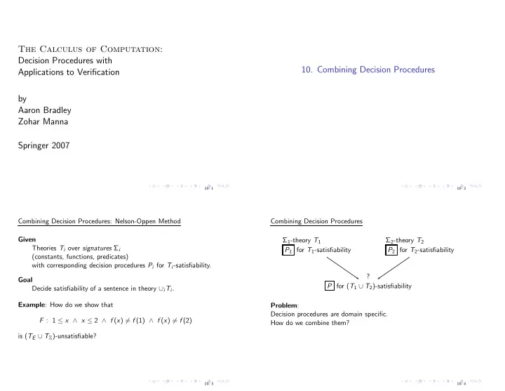
Combining Decision Procedures Σ1-theory T1 Σ2-theory T2 P1 for T1-satisfiability P2 for T2-satisfiability ? P for (T1 ∪ T2)-satisfiability Problem: Decision procedures are domain specific. How do we combine them?

10- 4

Nelson-Oppen Combination Method (N-O Method) Σ1 ∩ Σ2 = ∅ Σ1-theory T1 Σ2-theory T2 stably infinite stably infinite P1 for T1-satisfiability P2 for T2-satisfiability

• f quantifier-free Σ1-formulae
• f quantifier-free Σ2-formulae

P for (T1 ∪ T2)-satisfiability

• f quantifier-free (Σ1 ∪ Σ2)-formulae

10- 5

Nelson-Oppen: Limitations Given formula F in theory T1 ∪ T2.

• 1. F must be quantifier-free.
• 2. Signatures Σi of the combined theory only share =, i.e.,

Σ1 ∩ Σ2 = {=}

• 3. Theories must be stably infinite.

Note:

◮ Algorithm can be extended to combine arbitrary number of

theories Ti — combine two, then combine with another, and so on.

◮ We restrict F to be conjunctive formula — otherwise convert

to DNF and check each disjunct.

10- 6

Stably Infinite Theories A Σ-theory T is stably infinite iff for every quantifier-free Σ-formula F: if F is T-satisfiable then there exists some T-interpretation that satisfies F. Example: Σ-theory T Σ : {a, b, =} Axiom ∀x. x = a ∨ x = b For every T-interpretation I, |DI| ≤ 2 (at most two elements). Hence, T is not stably infinite. All the other theories mentioned so far are stably infinite.

10- 7

Example: Theory of partial orders Σ-theory T Σ : {, =} where is a binary predicate. Axioms

• 1. ∀x. x x

( reflexivity)

• 2. ∀x, y. x y ∧ y x → x = y

( antisymmetry)

• 3. ∀x, y, z. x y ∧ y z → x z

( transitivity)

10- 8

We prove T is stably infinite. Consider T-satisfiable quantifier-free Σ-formula F. Consider arbitrary satisfying T-interpretation I : (DI, αI), where αI maps to ≤I.

◮ Let A be any infinite set disjoint from DI ◮ Construct new interpretation J : (DJ, αJ)

◮ DJ = DI ∪ A ◮ αJ = { → ≤J}, where for a, b ∈ DJ,

a ≤J b def =

• a ≤I b

if a, b ∈ DI a = b

• therwise

J is T-interpretation satisfying F with infinite domain. Hence, T is stably infinite.

10- 9

Example: Consider quantifier-free conjunctive (ΣE ∪ ΣZ)-formula F : 1 ≤ x ∧ x ≤ 2 ∧ f (x) = f (1) ∧ f (x) = f (2) . The signatures of TE and TZ only share =. Also, both theories are stably infinite. Hence, the NO combination of the decision procedures for TE and TZ decides the (TE ∪ TZ)-satisfiability of F. Intuitively, F is (TE ∪ TZ)-unsatisfiable. For the first two literals imply x = 1 ∨ x = 2 so that f (x) = f (1) ∨ f (x) = f (2). Contradict last two literals. Hence, F is (TE ∪ TZ)-unsatisfiable.

10- 10

N-O Overview Phase 1: Variable Abstraction

◮ Given conjunction Γ in theory T1 ∪ T2. ◮ Convert to conjunction Γ1 ∪ Γ2 s.t.

◮ Γi in theory Ti ◮ Γ1 ∪ Γ2 satisfiable iff Γ satisfiable.

Phase 2: Check

◮ If there is some set S of equalities and disequalities between

the shared variables of Γ1 and Γ2 shared(Γ1, Γ2) = free(Γ1) ∩ free(Γ2) s.t. S ∪ Γi are Ti-satisfiable for all i, then Γ is satisfiable.

◮ Otherwise, unsatisfiable.

10- 11

Nelson-Oppen Method: Overview Consider quantifier-free conjunctive (Σ1 ∪ Σ2)-formula F. Two versions:

◮ nondeterministic — simple to present, but high complexity ◮ deterministic — efficient

Nelson-Oppen (N-O) method proceeds in two steps:

◮ Phase 1 (variable abstraction)

— same for both versions

◮ Phase 2

nondeterministic: guess equalities/disequalities and check deterministic: generate equalities/disequalities by equality propagation

10- 12

Phase 1: Variable abstraction Given quantifier-free conjunctive (Σ1 ∪ Σ2)-formula F. Transform F into two quantifier-free conjunctive formulae Σ1-formula F1 and Σ2-formula F2 s.t. F is (T1 ∪ T2)-satisfiable iff F1 ∧ F2 is (T1 ∪ T2)-satisfiable F1 and F2 are linked via a set of shared variables. For term t, let hd(t) be the root symbol, e.g. hd(f (x)) = f .

10- 13

Generation of F1 and F2 For i, j ∈ {1, 2} and i = j, repeat the transformations (1) if function f ∈ Σi and hd(t) ∈ Σj, F[f (t1, . . . , t, . . . , tn)] ⇒ F[f (t1, . . . , w, . . . , tn)] ∧ w = t (2) if predicate p ∈ Σi and hd(t) ∈ Σj, F[p(t1, . . . , t, . . . , tn)] ⇒ F[p(t1, . . . , w, . . . , tn)] ∧ w = t (3) if hd(s) ∈ Σi and hd(t) ∈ Σj, F[s = t] ⇒ F[⊤] ∧ w = s ∧ w = t (4) if hd(s) ∈ Σi and hd(t) ∈ Σj, F[s = t] ⇒ F[w1 = w2] ∧ w1 = s ∧ w2 = t where w, w1, and w2 are fresh variables.

10- 14

Example: Consider (ΣE ∪ ΣZ)-formula F : 1 ≤ x ∧ x ≤ 2 ∧ f (x) = f (1) ∧ f (x) = f (2) . According to transformation 1, since f ∈ ΣE and 1 ∈ ΣZ, replace f (1) by f (w1) and add w1 = 1. Similarly, replace f (2) by f (w2) and add w2 = 2. Now, the literals ΓZ : {1 ≤ x, x ≤ 2, w1 = 1, w2 = 2} are TZ-literals, while the literals ΓE : {f (x) = f (w1), f (x) = f (w2)} are TE-literals. Hence, construct the ΣZ-formula F1 : 1 ≤ x ∧ x ≤ 2 ∧ w1 = 1 ∧ w2 = 2 and the ΣE-formula F2 : f (x) = f (w1) ∧ f (x) = f (w2) . F1 and F2 share the variables {x, w1, w2}. F1 ∧ F2 is (TE ∪ TZ)-equisatisfiable to F.

10- 15

Example: Consider (ΣE ∪ ΣZ)-formula F : f (x) = x +y ∧ x ≤ y +z ∧ x +z ≤ y ∧ y = 1 ∧ f (x) = f (2) . In the first literal, hd(f (x)) = f ∈ ΣE and hd(x + y) = + ∈ ΣZ; thus, by (3), replace the literal with w1 = f (x) ∧ w1 = x + y . In the final literal, f ∈ ΣE but 2 ∈ ΣZ, so by (1), replace it with f (x) = f (w2) ∧ w2 = 2 . Now, separating the literals results in two formulae: F1 : w1 = x + y ∧ x ≤ y + z ∧ x + z ≤ y ∧ y = 1 ∧ w2 = 2 is a ΣZ-formula, and F2 : w1 = f (x) ∧ f (x) = f (w2) is a ΣE-formula. The conjunction F1 ∧ F2 is (TE ∪ TZ)-equisatisfiable to F.

10- 16

Nondeterministic Version

Phase 2: Guess and Check

◮ Phase 1 separated (Σ1 ∪ Σ2)-formula F into two formulae:

Σ1-formula F1 and Σ2-formula F2

◮ F1 and F2 are linked by a set of shared variables:

V = shared(F1, F2) = free(F1) ∩ free(F2)

◮ Let E be an equivalence relation over V . ◮ The arrangement α(V , E) of V induced by E is:

α(V , E) :

• u,v ∈ V . uEv

u = v ∧

• u,v ∈ V . ¬(uEv)

u = v Then, the original formula F is (T1 ∪ T2)-satisfiable iff there exists an equivalence relation E of V s.t. (1) F1 ∧ α(V , E) is T1-satisfiable, and (2) F2 ∧ α(V , E) is T2-satisfiable. Otherwise, F is (T1 ∪ T2)-unsatisfiable.

10- 17

Example: Consider (ΣE ∪ ΣZ)-formula F : 1 ≤ x ∧ x ≤ 2 ∧ f (x) = f (1) ∧ f (x) = f (2) Phase 1 separates this formula into the ΣZ-formula F1 : 1 ≤ x ∧ x ≤ 2 ∧ w1 = 1 ∧ w2 = 2 and the ΣE-formula F2 : f (x) = f (w1) ∧ f (x) = f (w2) with V = shared(F1, F2) = {x, w1, w2} There are 5 equivalence relations to consider, which we list by stating the partitions:

10- 18

• 1. {{x, w1, w2}}, i.e., x = w1 = w2:

x = w1 and f (x) = f (w1) ⇒ F2 ∧ α(V , E) is TE-unsatisfiable.

• 2. {{x, w1}, {w2}}, i.e., x = w1, x = w2:

x = w1 and f (x) = f (w1) ⇒ F2 ∧ α(V , E) is TE-unsatisfiable.

• 3. {{x, w2}, {w1}}, i.e., x = w2, x = w1:

x = w2 and f (x) = f (w2) ⇒ F2 ∧ α(V , E) is TE-unsatisfiable.

• 4. {{x}, {w1, w2}}, i.e., x = w1, w1 = w2:

w1 = w2 and w1 = 1 ∧ w2 = 2 ⇒ F1 ∧ α(V , E) is TZ-unsatisfiable.

• 5. {{x}, {w1}, {w2}}, i.e., x = w1, x = w2, w1 = w2:

x = w1 ∧ x = w2 and x = w1 = 1 ∨ x = w2 = 2 (since 1 ≤ x ≤ 2 implies that x = 1 ∨ x = 2 in TZ) ⇒ F1 ∧ α(V , E) is TZ-unsatisfiable. Hence, F is (TE ∪ TZ)-unsatisfiable.

10- 19

Example: Consider the (Σcons ∪ ΣZ)-formula F : car(x) + car(y) = z ∧ cons(x, z) = cons(y, z) . After two applications of (1), Phase 1 separates F into the Σcons-formula F1 : w1 = car(x) ∧ w2 = car(y) ∧ cons(x, z) = cons(y, z) and the ΣZ-formula F2 : w1 + w2 = z , with V = shared(F1, F2) = {z, w1, w2} . Consider the equivalence relation E given by the partition {{z}, {w1}, {w2}} . The arrangement α(V , E) : z = w1 ∧ z = w2 ∧ w1 = w2 satisfies both F1 and F2: F1 ∧ α(V , E) is Tcons-satisfiable, and F2 ∧ α(V , E) is TZ-satisfiable. Hence, F is (Tcons ∪ TZ)-satisfiable.

10- 20

Practical Efficiency Phase 2 was formulated as “guess and check”: First, guess an equivalence relation E, then check the induced arrangement. The number of equivalence relations grows super-exponentially with the # of shared variables. It is given by Bell numbers. e.g., 12 shared variables ⇒ over four million equivalence relations. Solution: Deterministic Version

10- 21

Deterministic Version

Phase 1 as before Phase 2 asks the decision procedures P1 and P2 to propagate new equalities. Example 1: Real linear arithmethic TR Theory of equality TE PR PE F : f (f (x)−f (y)) = f (z) ∧ x ≤ y ∧ y + z ≤ x ∧ 0 ≤ z (TR ∪ TE)-unsatisfiable Intuitively, last 3 conjuncts ⇒ x = y ∧ z = 0 contradicts 1st conjunct

10- 22

Phase 1: Variable Abstraction F : f (f (x) − f (y)) = f (z) ∧ x ≤ y ∧ y + z ≤ x ∧ 0 ≤ z f (x) ⇒ u f (y) ⇒ v u − v ⇒ w ΓE : {f (w) = f (z), u = f (x), v = f (y)} . . . TE-formula ΓR : {x ≤ y, y + z ≤ x, 0 ≤ z, w = u − v} . . . TR-formula shared(ΓR, ΓE) = {x, y, z, u, v, w} Nondeterministic version — over 200 Es! Let’s try the deterministic version.

10- 23

Phase 2: Equality Propagation PR s0 : ΓR, ΓE, {} PE ΓR | = x = y s1 : ΓR, ΓE, {x = y} ΓE ∪ {x = y} | = u = v s2 : ΓR, ΓE, {x = y, u = v} ΓR ∪ {u = v} | = z = w s3 : ΓR, ΓE, {x = y, u = v, z = w} ΓE ∪ {z = w} | = false s4 : false

• Contradiction. Thus, F is (TR ∪ TE)-unsatisfiable.

If there were no contradiction, F would be (TR ∪ TE)-satisfiable.

10- 24

Convex Theories Claim: Equality propagation is a decision procedure for convex theories.

• Def. A Σ-theory T is convex iff

for every quantifier-free conjunction Σ-formula F and for every disjunction

n

• i=1

(ui = vi) if F | =

n

• i=1

(ui = vi) then F | = ui = vi, for some i ∈ {1, . . . , n}

10- 25

Convex Theories

◮ TE, TR, TQ, Tcons are convex ◮ TZ, TA are not convex

Example: TZ is not convex Consider quantifier-free conjunctive F : 1 ≤ z ∧ z ≤ 2 ∧ u = 1 ∧ v = 2 Then F | = z = u ∨ z = v but F | = z = u F | = z = v

10- 26

Example: The theory of arrays TA is not convex. Consider the quantifier-free conjunctive ΣA-formula F : ai ⊳ v[j] = v . Then F ⇒ i = j ∨ a[j] = v , but F ⇒ i = j F ⇒ a[j] = v .

10- 27

What if T is Not Convex? Case split when: Γ | =

n

• i=1

(ui = vi) but Γ | = ui = vi for all i = 1, . . . , n

◮ For each i = 1, . . . , n, construct a branch on which

ui = vi is assumed.

◮ If all branches are contradictory, then unsatisfiable.

Otherwise, satisfiable. · . . . . . . . . . u1 = v1 ui = vi un = vn

10- 28

Example 2: Non-Convex Theory TZ not convex! TE convex PZ PE Γ : 1 ≤ x, x ≤ 2, f (x) = f (1), f (x) = f (2)

• in TZ ∪ TE

◮ Replace f (1) by f (w1), and add w1 = 1. ◮ Replace f (2) by f (w2), and add w2 = 2.

Result: ΓZ =        1 ≤ x, x ≤ 2, w1 = 1, w2 = 2        and ΓE = f (x) = f (w1), f (x) = f (w2)

• shared(ΓZ, ΓE) = {x, w1, w2}

10- 29

Example 2: Non-Convex Theory s0 : ΓZ, ΓE, {} ⋆ s1 : ΓZ, ΓE, {x = w1} s3 : ΓZ, ΓE, {x = w2} s2 : ⊥ s4 : ⊥ x = w1 ΓE ∪ {x = w1} | = ⊥ x = w2 ΓE ∪ {x = w2} | = ⊥ ⋆ : ΓZ | = x = w1 ∨ x = w2 All leaves are labeled with ⊥ ⇒ Γ is (TZ ∪ TE)-unsatisfiable.

10- 30

Example 3: Non-Convex Theory Γ :

• 1 ≤ x,

x ≤ 3, f (x) = f (1), f (x) = f (3), f (1) = f (2)

• in TZ ∪ TE

◮ Replace f (1) by f (w1), and add w1 = 1. ◮ Replace f (2) by f (w2), and add w2 = 2. ◮ Replace f (3) by f (w3), and add w3 = 3.

Result: ΓZ =            1 ≤ x, x ≤ 3, w1 = 1, w2 = 2, w3 = 3            and ΓE =    f (x) = f (w1), f (x) = f (w3), f (w1) = f (w2)    shared(ΓZ, ΓE) = {x, w1, w2, w3}

10- 31

Example 3: Non-Convex Theory s0 : ΓZ, ΓE, {} ⋆ s1 : ΓZ, ΓE, {x = w1} s3 : ΓZ, ΓE, {x = w2} s5 : ΓZ, ΓE, {x = w3} s2 : ⊥ s6 : ⊥ x = w1 ΓE ∪ {x = w1} | = ⊥ x = w2 x = w3 ΓE ∪ {x = w3} | = ⊥ ⋆ : ΓZ | = x = w1 ∨ x = w2 ∨ x = w3 No more equations on middle leaf ⇒ Γ is (TZ ∪ TE)-satisfiable.

10- 32