The Calculus of Computation: Decision Procedures with 9. - - PowerPoint PPT Presentation

The Calculus of Computation: Decision Procedures with Applications to Verification by Aaron Bradley Zohar Manna Springer 2007

9- 1

• 9. Quantifier-free Equality and Data Structures

9- 2

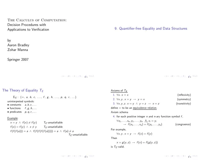
The Theory of Equality TE

ΣE : {=, a, b, c, . . . , f , g, h, . . . , p, q, r, . . .} uninterpreted symbols:

• constants

a, b, c, . . .

• functions

f , g, h, . . .

• predicates

p, q, r, . . . Example: x = y ∧ f (x) = f (y) TE-unsatisfiable f (x) = f (y) ∧ x = y TE-unsatisfiable f (f (f (a))) = a ∧ f (f (f (f (f (a))))) = a ∧ f (a) = a TE-unsatisfiable

9- 3

Axioms of TE

• 1. ∀x. x = x

(reflexivity)

• 2. ∀x, y. x = y → y = x

(symmetry)

• 3. ∀x, y, z. x = y ∧ y = z → x = z

(transitivity) define = to be an equivalence relation. Axiom schema

• 4. for each positive integer n and n-ary function symbol f ,

∀x1, . . . , xn, y1, . . . , yn.

i xi = yi

→ f (x1, . . . , xn) = f (y1, . . . , yn) (congruence) For example, ∀x, y. x = y → f (x) = f (y) Then x = g(y, z) → f (x) = f (g(y, z)) is TE-valid.

9- 4

Axiom schema

• 5. for each positive integer n and n-ary predicate symbol p,

∀x1, . . . , xn, y1, . . . , yn.

• i

xi = yi → (p(x1, . . . , xn) ↔ p(y1, . . . , yn)) (equivalence) Thus, x = y → (p(x) ↔ p(y)) is TE-valid.

9- 5

We discuss TE-formulae without predicates For example, for ΣE-formula F : p(x) ∧ q(x, y) ∧ q(y, z) → ¬q(x, z) introduce fresh constant • and fresh functions fp and fg, and transform F to G : fp(x) = • ∧ fq(x, y) = • ∧ fq(y, z) = • → fq(x, z) = • .

9- 6

Equivalence and Congruence Relations: Basics

Binary relation R over set S

• is an equivalence relation if

◮ reflexive: ∀s ∈ S. sRs; ◮ symmetric: ∀s1, s2 ∈ S. s1Rs2 → s2Rs1; ◮ transitive: ∀s1, s2, s3 ∈ S. s1Rs2 ∧ s2Rs3 → s1Rs3.

Example: Define the binary relation ≡2 over the set Z of integers m ≡2 n iff (m mod 2) = (n mod 2) That is, m, n ∈ Z are related iff they are both even or both odd. ≡2 is an equivalence relation

• is a congruence relation if in addition

∀s, t.

n

• i=1

siRti → f (s)Rf (t) .

9- 7

Classes For equivalence congruence

• relation R over set S,

The equivalence congruence

• class of s ∈ S under R is

[s]R

def

= {s′ ∈ S : sRs′} . Example: The equivalence class of 3 under ≡2 over Z is [3]≡2 = {n ∈ Z : n is odd} . Partitions A partition P of S is a set of subsets of S that is

◮ total S′∈P

S′

• = S

◮ disjoint

∀S1, S2 ∈ P. S1 ∩ S2 = ∅

9- 8

Quotient The quotient S/R of S by equivalence congruence

• relation R is the set of

equivalence congruence

• classes

S/R = {[s]R : s ∈ S} . It is a partition Example: The quotient Z/ ≡2 is a partition of Z. The set of equivalence classes {{n ∈ Z : n is odd}, {n ∈ Z : n is even}} Note duality between relations and classes

9- 9

Refinements Two binary relations R1 and R2 over set S. R1 is refinement of R2, R1 ≺ R2, if ∀s1, s2 ∈ S. s1R1s2 → s1R2s2 . R1 refines R2. Examples:

◮ For S = {a, b},

R1 : {aR1b} R2 : {aR2b, bR2b} Then R1 ≺ R2

◮ For set S,

R1 induced by the partition P1 : {{s} : s ∈ S} R2 induced by the partition P2 : {S} Then R1 ≺ R2.

◮ For set Z

R1 : {xR1y : x mod 2 = y mod 2} R2 : {xR2y : x mod 4 = y mod 4} Then R2 ≺ R1.

9- 10

Closures Given binary relation R over S. The equivalence closure RE of R is the equivalence relation s.t.

◮ R refines RE, i.e. R ≺ RE; ◮ for all other equivalence relations R′ s.t. R ≺ R′,

either R′ = RE or RE ≺ R′ That is, RE is the “smallest” equivalence relation that “covers” R. Example: If S = {a, b, c, d} and R = {aRb, bRc, dRd}, then

• aRb, bRc, dRd ∈ RE

since R ⊆ RE;

• aRa, bRb, cRc ∈ RE

by reflexivity;

• bRa, cRb ∈ RE

by symmetry;

• aRc ∈ RE

by transitivity;

• cRa ∈ RE

by symmetry. Hence, RE = {aRb, bRa, aRa, bRb, bRc, cRb, cRc, aRc, cRa, dRd} . Similarly, the congruence closure RC of R is the “smallest” congruence relation that “covers” R.

9- 11

Congruence Closure Algorithm

Given ΣE-formula F : s1 = t1 ∧ · · · ∧ sm = tm ∧ sm+1 = tm+1 ∧ · · · ∧ sn = tn decide if F is ΣE-satisfiable. Definition: For ΣE-formula F, the subterm set SF of F is the set that contains precisely the subterms of F. Example: The subterm set of F : f (a, b) = a ∧ f (f (a, b), b) = a is SF = {a, b, f (a, b), f (f (a, b), b)} .

9- 12

The Algorithm Given ΣE-formula F F : s1 = t1 ∧ · · · ∧ sm = tm ∧ sm+1 = tm+1 ∧ · · · ∧ sn = tn with subterm set SF, F is TE-satisfiable iff there exists a congruence relation ∼ over SF such that

◮ for each i ∈ {1, . . . , m}, si ∼ ti; ◮ for each i ∈ {m + 1, . . . , n}, si ∼ ti.

Such congruence relation ∼ defines TE-interpretation I : (DI, αI)

• f F. DI consists of |SF/ ∼ | elements, one for each congruence

class of SF under ∼. Instead of writing I | = F for this TE-interpretation, we abbreviate ∼ | = F The goal of the algorithm is to construct the congruence relation

• f SF, or to prove that no congruence relation exists.

9- 13

F : s1 = t1 ∧ · · · ∧ sm = tm

• generate congruence closure

∧ sm+1 = tm+1 ∧ · · · ∧ sn = tn

• search for contradiction

The algorithm performs the following steps:

• 1. Construct the congruence closure ∼ of

{s1 = t1, . . . , sm = tm}

• ver the subterm set SF. Then

∼ | = s1 = t1 ∧ · · · ∧ sm = tm .

• 2. If for any i ∈ {m + 1, . . . , n}, si ∼ ti, return unsatisfiable.
• 3. Otherwise, ∼|

= F, so return satisfiable. How do we actually construct the congruence closure in Step 1?

9- 14

Initially, begin with the finest congruence relation ∼0 given by the partition {{s} : s ∈ SF} . That is, let each term of SF be its own congruence class. Then, for each i ∈ {1, . . . , m}, impose si = ti by merging the congruence classes [si]∼i−1 and [ti]∼i−1 to form a new congruence relation ∼i. To accomplish this merging,

◮ form the union of [si]∼i−1 and [ti]∼i−1 ◮ propagate any new congruences that arise within this union.

The new relation ∼i is a congruence relation in which si ∼ ti.

9- 15

Example: Given ΣE-formula F : f (a, b) = a ∧ f (f (a, b), b) = a Construct initial partition by letting each member of the subterm set SF be its own class:

• 1. {{a}, {b}, {f (a, b)}, {f (f (a, b), b)}}

According to the first literal f (a, b) = a, merge {f (a, b)} and {a} to form partition

• 2. {{a, f (a, b)}, {b}, {f (f (a, b), b)}}

According to the (congruence) axiom, f (a, b) ∼ a, b ∼ b implies f (f (a, b), b) ∼ f (a, b) , resulting in the new partition

• 3. {{a, f (a, b), f (f (a, b), b)}, {b}}

This partition represents the congruence closure of SF. Now, is it the case that

• 4. {{a, f (a, b), f (f (a, b), b)}, {b}} |

= F ? No, as f (f (a, b), b) ∼ a but F asserts that f (f (a, b), b) = a. Hence, F is TE-unsatisfiable.

9- 16

Example: Given ΣE-formula F : f (f (f (a))) = a ∧ f (f (f (f (f (a))))) = a ∧ f (a) = a From the subterm set SF, the initial partition is

• 1. {{a}, {f (a)}, {f 2(a)}, {f 3(a)}, {f 4(a)}, {f 5(a)}}

where, for example, f 3(a) abbreviates f (f (f (a))). According to the literal f 3(a) = a, merge {f 3(a)} and {a} . From the union,

• 2. {{a, f 3(a)}, {f (a)}, {f 2(a)}, {f 4(a)}, {f 5(a)}}

deduce the following congruence propagations: f 3(a) ∼ a ⇒ f (f 3(a)) ∼ f (a) i.e. f 4(a) ∼ f (a) and f 4(a) ∼ f (a) ⇒ f (f 4(a)) ∼ f (f (a)) i.e. f 5(a) ∼ f 2(a) Thus, the final partition for this iteration is the following:

• 3. {{a, f 3(a)}, {f (a), f 4(a)}, {f 2(a), f 5(a)}} .

9- 17

• 3. {{a, f 3(a)}, {f (a), f 4(a)}, {f 2(a), f 5(a)}} .

From the second literal, f 5(a) = a, merge {f 2(a), f 5(a)} and {a, f 3(a)} to form the partition

• 4. {{a, f 2(a), f 3(a), f 5(a)}, {f (a), f 4(a)}} .

Propagating the congruence f 3(a) ∼ f 2(a) ⇒ f (f 3(a)) ∼ f (f 2(a)) i.e. f 4(a) ∼ f 3(a) yields the partition

• 5. {{a, f (a), f 2(a), f 3(a), f 4(a), f 5(a)}} ,

which represents the congruence closure in which all of SF are

• equal. Now,
• 6. {{a, f (a), f 2(a), f 3(a), f 4(a), f 5(a)}} |

= F ? No, as f (a) ∼ a, but F asserts that f (a) = a. Hence, F is TE-unsatisfiable.

9- 18

Example: Given ΣE-formula F : f (x) = f (y) ∧ x = y . The subterm set SF induces the following initial partition:

• 1. {{x}, {y}, {f (x)}, {f (y)}} .

Then f (x) = f (y) indicates to merge {f (x)} and {f (y)} . The union {f (x), f (y)} does not yield any new congruences, so the final partition is

• 2. {{x}, {y}, {f (x), f (y)}} .

Does

• 3. {{x}, {y}, {f (x), f (y)}} |

= F ? Yes, as x ∼ y, agreeing with x = y. Hence, F is TE-satisfiable.

9- 19

Directed Acyclic Graph (DAG) For ΣE-formula F, graph-based data structure for representing the subterms of SF (and congruence relation between them). 1 : f 2 : f 3 : a 4 : b f (f (a, b), b) f (a, b) a b Efficient way for computing the congruence closure algorithm.

9- 20

TE-Satisfiability (Summary of idea) f (a, b) = a ∧ f (f (a, b), b) = a 1 : f 2 : f 3 : a 4 : b 1 : f 2 : f 3 : a 4 : b 1 : f 2 : f 3 : a 4 : b Initial DAG f (a, b) = a ⇒ merge f (a, b) a explicit equation f (a, b) ∼ a, b ∼ b ⇒ f (f (a, b), b) ∼ f (a, b) merge f (f (a, b), b) f (a, b) by congruence find f (f (a, b), b) = a = find a f (f (a, b), b) = a

• ⇒ Unsatisfiable

9- 21

DAG representation type node = { id : id node’s unique identification number fn : string constant or function name args : id list list of function arguments mutable find : id the representative of the congruence class mutable ccpar : id set if the node is the representative for its congruence class, then its ccpar (congruence closure parents) are all parents of nodes in its congruence class }

9- 22

DAG Representation of node 2 type node = { id : id fn : string args : idlist mutable find : id mutable ccpar : idset } . . . 2 . . . f . . . [3, 4] . . . 3 . . . ∅ 1 : f 2 : f 3 : a 4 : b

9- 23

DAG Representation of node 3 type node = { id : id fn : string args : idlist mutable find : id mutable ccpar : idset } . . . 3 . . . a . . . [] . . . 3 . . . {1, 2} 1 : f 2 : f 3 : a 4 : b

9- 24

The Implementation

find function returns the representative of node’s congruence class let rec find i = let n = node i in if n.find = i then i else find n.find 1 : f 2 : f 3 : a 4 : b Example: find 2 = 3 find 3 = 3 3 is the representative of 2.

9- 25

union function let union i1 i2 = let n1 = node (find i1) in let n2 = node (find i2) in n1.find ← n2.find; n2.ccpar ← n1.ccpar ∪ n2.ccpar; n1.ccpar ← ∅ n2 is the representative of the union class

9- 26

Example 1 : f 2 : f 3 : a 4 : b union 1 2 n1 = 1 n2 = 3 1.find ← 3 3.ccpar ← {1, 2} 1.ccpar ← ∅

9- 27

ccpar function Returns parents of all nodes in i’s congruence class let ccpar i = (node (find i)).ccpar congruent predicate Test whether i1 and i2 are congruent let congruent i1 i2 = let n1 = node i1 in let n2 = node i2 in n1.fn = n2.fn ∧ |n1.args| = |n2.args| ∧ ∀i ∈ {1, . . . , |n1.args|}. find n1.args[i] = find n2.args[i]

9- 28

Example: 1 : f 2 : f 3 : a 4 : b Are 1 and 2 congruent? fn fields — both f # of arguments — same left arguments f (a, b) and a — both congruent to 3 right arguments b and b — both 4 (congruent) Therefore 1 and 2 are congruent.

9- 29

merge function let rec merge i1 i2 = if find i1 = find i2 then begin let Pi1 = ccpar i1 in let Pi2 = ccpar i2 in union i1 i2; foreach t1, t2 ∈ Pi1 × Pi2 do if find t1 = find t2 ∧ congruent t1 t2 then merge t1 t2 done end Pi1 and Pi2 store the current values of ccpar i1 and ccpar i2.

9- 30

Decision Procedure: TE-satisfiability Given ΣE-formula F : s1 = t1 ∧ · · · ∧ sm = tm ∧ sm+1 = tm+1 ∧ · · · ∧ sn = tn , with subterm set SF, perform the following steps:

• 1. Construct the initial DAG for the subterm set SF.
• 2. For i ∈ {1, . . . , m}, merge si ti.
• 3. If find si = find ti for some i ∈ {m + 1, . . . , n}, return

unsatisfiable.

• 4. Otherwise (if find si = find ti for all i ∈ {m + 1, . . . , n})

return satisfiable.

9- 31

Example 1: TE-Satisfiability f (a, b) = a ∧ f (f (a, b), b) = a (1) 1 : f 2 : f 3 : a 4 : b (2) 1 : f 2 : f 3 : a 4 : b (3) 1 : f 2 : f 3 : a 4 : b Initial DAG merge 2 3 union 2 3 P2 = {1} P3 = {2} congruent 1 2 merge 1 2 union 1 2 P1 = {} P2 = {1, 2} find f (f (a, b), b) = a = find a ⇒ Unsatisfiable

9- 32

Given ΣE-formula F : f (a, b) = a ∧ f (f (a, b), b) = a . The subterm set is SF = {a, b, f (a, b), f (f (a, b), b)} , resulting in the initial partition (1) {{a}, {b}, {f (a, b)}, {f (f (a, b), b)}} in which each term is its own congruence class. Fig (1). Final partition (2) {{a, f (a, b), f (f (a, b), b)}, {b}} Note: dash edge merge dictated by equalities in F dotted edge deduced merge Does (3) {{a, f (a, b), f (f (a, b), b)}, {b}} | = F ? No, as f (f (a, b), b) ∼ a, but F asserts that f (f (a, b), b) = a. Hence, F is TE-unsatisfiable.

9- 33

Example 2: TE-Satisfiability f (f (f (a))) = a ∧ f (f (f (f (f (a))))) = a ∧ f (a) = a 5 : f 4 : f 3 : f 2 : f 1 : f 0 : a (1) Initial DAG 5 : f 4 : f 3 : f 2 : f 1 : f 0 : a (2) f (f (f (a))) = a ⇒ merge 3 0 P3 = {4} P0 = {1} ⇒ merge 4 1 P4 = {5} P1 = {2} ⇒ merge 5 2 P5 = {} P2 = {3}

9- 34

Example 2: TE-Satisfiability f (f (f (a))) = a ∧ f (f (f (f (f (a))))) = a ∧ f (a) = a 5 : f 4 : f 3 : f 2 : f 1 : f 0 : a (2) 5 : f 4 : f 3 : f 2 : f 1 : f 0 : a (3) f (f (f (f (f (a))))) = a ⇒ merge 5 0 P5 = {3} P0 = {1, 4} ⇒ merge 3 1

• STOP. Why?

find f (a) = f (a) = find a ⇒ Unsatisfiable

9- 35

Given ΣE-formula F : f (f (f (a))) = a ∧ f (f (f (f (f (a))))) = a ∧ f (a) = a , which induces the initial partition

• 1. {{a}, {f (a)}, {f 2(a)}, {f 3(a)}, {f 4(a)}, {f 5(a)}} .

The equality f 3(a) = a induces the partition

• 2. {{a, f 3(a)}, {f (a), f 4(a)}, {f 2(a), f 5(a)}} .

The equality f 5(a) = a induces the partition

• 3. {{a, f (a), f 2(a), f 3(a), f 4(a), f 5(a)}} .

Now, does {{a, f (a), f 2(a), f 3(a), f 4(a), f 5(a)}} | = F ? No, as f (a) ∼ a, but F asserts that f (a) = a. Hence, F is TE-unsatisfiable.

9- 36

Theorem (Sound and Complete) Quantifier-free conjunctive ΣE-formula F is TE-satisfiable iff the congruence closure algorithm returns satisfiable.

9- 37

Recursive Data Structures

Quantifier-free Theory of Lists Tcons Σcons : {cons, car, cdr, atom, =}

• constructor cons

: cons(a, b) list constructed by prepending a to b

• left projector car

: car(cons(a, b)) = a

• right projector cdr : cdr(cons(a, b)) = b
• atom

: unary predicate

9- 38

Axioms of Tcons

◮ reflexivity, symmetry, transitivity ◮ congruence axioms:

∀x1, x2, y1, y2. x1 = x2 ∧ y1 = y2 → cons(x1, y1) = cons(x2, y2) ∀x, y. x = y → car(x) = car(y) ∀x, y. x = y → cdr(x) = cdr(y)

◮ equivalence axiom:

∀x, y. x = y → (atom(x) ↔ atom(y))

◮

(A1) ∀x, y. car(cons(x, y)) = x (left projection) (A2) ∀x, y. cdr(cons(x, y)) = y (right projection) (A3) ∀x. ¬atom(x) → cons(car(x), cdr(x)) = x (construction) (A4) ∀x, y. ¬atom(cons(x, y)) (atom)

9- 39

Simplifications

◮ Consider only quantifier-free conjunctive Σcons-formulae.

Convert non-conjunctive formula to DNF and check each disjunct.

◮ ¬atom(ui) literals are removed:

replace ¬atom(ui) with ui = cons(u1

i , u2 i )

by the (construnction) axiom.

◮ Because of similarity to ΣE, we sometimes combine

Σcons ∪ ΣE.

9- 40

Algorithm: Tcons-Satisfiability (the idea) F : s1 = t1 ∧ · · · ∧ sm = tm

• generate congruence closure

∧ sm+1 = tm+1 ∧ · · · ∧ sn = tn

• search for contradiction

∧ atom(u1) ∧ · · · ∧ atom(uℓ)

• search for contradiction

where si, ti, and ui are Tcons-terms

9- 41

Algorithm: Tcons-Satisfiability

• 1. Construct the initial DAG for SF
• 2. for each node n with n.fn = cons

◮ add car(n) and merge car(n) n.args[1] ◮ add cdr(n) and merge cdr(n) n.args[2]

by axioms (A1), (A2)

• 3. for 1 ≤ i ≤ m, merge si ti
• 4. for m + 1 ≤ i ≤ n, if find si = find ti, return unsatisfiable
• 5. for 1 ≤ i ≤ ℓ, if ∃v. find v = find ui ∧ v.fn = cons,

return unsatisfiable

• 6. Otherwise, return satisfiable

car cdr cons x y

9- 42

Example: Given (Σcons ∪ ΣE)-formula F : car(x) = car(y) ∧ cdr(x) = cdr(y) ∧ ¬atom(x) ∧ ¬atom(y) ∧ f (x) = f (y) where the function symbol f is in ΣE F ′ : car(x) = car(y) ∧ (1) cdr(x) = cdr(y) ∧ (2) x = cons(u1, v1) ∧ (3) y = cons(u2, v2) ∧ (4) f (x) = f (y) (5) Recall the projection axioms: (A1) ∀x, y. car(cons(x, y)) = x (A2) ∀x, y. cdr(cons(x, y)) = y

9- 43

Example(cont): Initial DAG car f cdr car f cdr x y car cdr car cdr cons cons u1 v1 u2 v2 axioms (A1), (A2)

9- 44

Example(cont): merge car f cdr car f cdr x y car cdr car cdr cons cons u1 v1 u2 v2 (1) (2) (3)

explicit equation by congruence 1 : merge car(x) car(y) 2 : merge cdr(x) cdr(y) 3 : merge x cons(u1, v1) ⇓

9- 45

Example(cont): Propagation car f cdr car f cdr x y car cdr car cdr cons cons u1 v1 u2 v2 3A 3B

Congruent: car(x) car(cons(u1, v1)) find car(x) = car(y) find car(cons(. . .)) = u1 Congruent: cdr(x) cdr(cons(u1, v1)) find cdr(x) = cdr(y) find cdr(cons(. . .)) = v1

9- 46

Example(cont): merge car f cdr car f cdr x y car cdr car cdr cons cons u1 v1 u2 v2 (4) 4A 4B

4 : merge y cons(u2, v2) ⇓ Congruent: car(y) car(cons(u2, v2)) find car(y) = u1 find car(cons(. . .)) = u2 Congruent: cdr(y) cdr(cons(u2, v2)) find cdr(y) = v1 find cdr(cons(. . .)) = v2 ⇓

9- 47

Example(cont): congruence car f cdr car f cdr x y car cdr car cdr cons cons u1 v1 u2 v2 4C 4D

Congruent: cons(u1, v1) cons(u2, v2) Congruent: f (x) f (y) 5 : find f (x) = f (y) find f (y) = f (y) ⇓ F is unsatisfiable

9- 48

Arrays

(1) Quantifier-free Fragment of TA ΣA : {·[·], ·· ⊳ ·, =} , where

◮ a[i] is a binary function representing

read of array a at index i;

◮ ai ⊳ v is a ternary function representing

write of value v to index i of array a;

◮ = is a binary predicate.

Axioms of TA:

• 1. axioms of (reflexivity), (symmetry), and (transitivity) of TE
• 2. ∀a, i, j. i = j → a[i] = a[j]

(array congruence)

• 3. ∀a, v, i, j. i = j → ai ⊳ v[j] = v

(read-over-write 1)

• 4. ∀a, v, i, j. i = j → ai ⊳ v[j] = a[j]

(read-over-write 2) Note: a may itself be a write term, e.g., ai′ ⊳ v ′. Then (ai′ ⊳ v ′)i ⊳ v means: first write the value v ′ to index i′ of a then write the value v to index i of a

9- 49

The Decision Procedure Given quantifier-free conjunctive ΣA-formula F. To decide the TA-satisfiability of F: Step 1 If F does not contain any write terms ai ⊳ v, then

• 1. associate array variables a with fresh function symbol fa, and

replace read terms a[i] with fa(i);

• 2. decide the TE-satisfiability of the resulting formula.

9- 50

Step 2 Select some read-over-write term ai ⊳ v[j] (note that a may itself be a write term) and split on two cases:

• 1. According to (read-over-write 1), replace

F[ai ⊳ v[j]] with F1 : F[v] ∧ i = j , and recurse on F1. If F1 is found to be TA-satisfiable, return satisfiable.

• 2. According to (read-over-write 2), replace

F[ai ⊳ v[j]] with F2 : F[a[j]] ∧ i = j , and recurse on F2. If F2 is found to be TA-satisfiable, return satisfiable. If both F1 and F2 are found to be TA-unsatisfiable, return unsatisfiable.

9- 51

Example: Consider ΣA-formula F : i1 = j ∧ i1 = i2 ∧ a[j] = v1 ∧ ai1 ⊳ v1i2 ⊳ v2[j] = a[j] . F contains a write term, ai1 ⊳ v1i2 ⊳ v2[j] = a[j] . According to (read-over-write 1), assume i2 = j and recurse on F1 : i2 = j ∧ i1 = j ∧ i1 = i2 ∧ a[j] = v1 ∧ v2 = a[j] . F1 does not contain any write terms, so rewrite it to F ′

1 : i2 = j ∧ i1 = j ∧ i1 = i2 ∧ fa(j) = v1 ∧ v2 = fa(j) .

The first two literals imply that i1 = i2, contradicting the third literal, so F ′

1 is TE-unsatisfiable.

9- 52

Returning, we try the second case: according to (read-over-write 2), assume i2 = j and recurse on F2 : i2 = j ∧ i1 = j ∧ i1 = i2 ∧ a[j] = v1 ∧ ai1 ⊳ v1[j] = a[j] . F2 contains a write term. According to (read-over-write 1), assume i1 = j and recurse on F3 : i1 = j ∧ i2 = j ∧ i1 = j ∧ i1 = i2 ∧ a[j] = v1 ∧ v1 = a[j] . Contradiction because of the final two terms. Thus, according to (read-over-write 2), assume i1 = j and recurse on F4 : i1 = j ∧ i2 = j ∧ i1 = j ∧ i1 = i2 ∧ a[j] = v1 ∧ a[j] = a[j] . Two contradictions: the first and third literals contradict each

• ther, and the final literal is contradictory. As all branches have

been tried, F is TA-unsatisfiable. Suppose instead that F does not contain the literal i1 = i2. Is this new formula TA-satisfiable?

9- 53