The Calculus of Computation: Decision Procedures with 5. Program - - PowerPoint PPT Presentation

The Calculus of Computation: Decision Procedures with Applications to Verification by Aaron Bradley Zohar Manna Springer 2007

5- 1

• 5. Program Correctness: Mechanics

5- 2

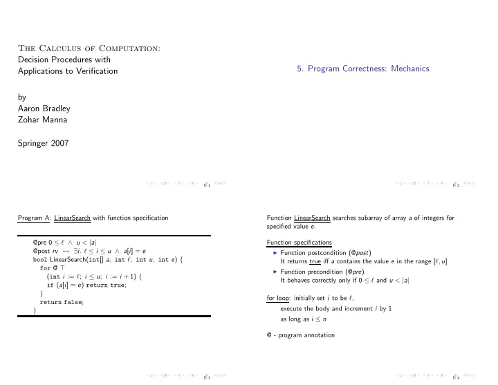
Program A: LinearSearch with function specification @pre 0 ≤ ℓ ∧ u < |a| @post rv ↔ ∃i. ℓ ≤ i ≤ u ∧ a[i] = e bool LinearSearch(int[] a, int ℓ, int u, int e) { for @ ⊤ (int i := ℓ; i ≤ u; i := i + 1) { if (a[i] = e) return true; } return false; }

5- 3

Function LinearSearch searches subarray of array a of integers for specified value e. Function specifications

◮ Function postcondition (@post)

It returns true iff a contains the value e in the range [ℓ, u]

◮ Function precondition (@pre)

It behaves correctly only if 0 ≤ ℓ and u < |a| for loop: initially set i to be ℓ, execute the body and increment i by 1 as long as i ≤ n @ - program annotation

5- 4

Program B: BinarySearch with function specification @pre 0 ≤ ℓ ∧ u < |a| ∧ sorted(a, ℓ, u) @post rv ↔ ∃i. ℓ ≤ i ≤ u ∧ a[i] = e bool BinarySearch(int[] a, int ℓ, int u, int e) { if (ℓ > u) return false; else { int m := (ℓ + u) div 2; if (a[m] = e) return true; else if (a[m] < e) return BinarySearch(a, m + 1, u, e); else return BinarySearch(a, ℓ, m − 1, e); } }

5- 5

The recursive function BinarySearch searches subarray of sorted array a of integers for specified value e. sorted: weakly increasing order, i.e. sorted(a, ℓ, u) ⇔ ∀i, j. ℓ ≤ i ≤ j ≤ u → a[i] ≤ a[j] Defined in the combined theory of integers and arrays, TZ∪A Function specifications

◮ Function postcondition (@post)

It returns true iff a contains the value e in the range [ℓ, u]

◮ Function precondition (@pre)

It behaves correctly only if 0 ≤ ℓ and u < |a|

5- 6

Program C: BubbleSort with function specification @pre ⊤ @post sorted(rv, 0, |rv| − 1) int[] BubbleSort(int[] a0) { int[] a := a0; for @ ⊤ (int i := |a| − 1; i > 0; i := i − 1) { for @ ⊤ (int j := 0; j < i; j := j + 1) { if (a[j] > a[j + 1]) { int t := a[j]; a[j] := a[j + 1]; a[j + 1] := t; } } } return a; }

5- 7

Function BubbleSort sorts integer array a

a: unsorted sorted

largest by “bubbling” the largest element of the left unsorted region of a toward the sorted region on the right. Each iteration of the outer loop expands the sorted region by one cell.

5- 8

Sample execution of BubbleSort

2 3 4 1 2 5 6 j i 2 3 4 1 2 5 6 j i 2 3 4 1 2 5 6 j i 2 3 1 4 2 5 6 j i 2 3 1 2 4 5 6 j, i 2 3 1 2 4 5 6 j i

5- 9

Program Annotation

◮ Function Specifications

function postcondition (@post) function precondition (@pre)

◮ Runtime Assertions

e.g., @ 0 ≤ j < |a| ∧ 0 ≤ j + 1 < |a| a[j] := a[j + 1]

◮ Loop Invariants

e.g., @ L : ℓ ≤ i ∧ ∀j. ℓ ≤ j < i → a[j] = e

5- 10

Program A: LinearSearch with runtime assertions @pre ⊤ @post ⊤ bool LinearSearch(int[] a, int ℓ, int u, int e) { for @ ⊤ (int i := ℓ; i ≤ u; i := i + 1) { @ 0 ≤ i < |a|; if (a[i] = e) return true; } return false; }

5- 11

Program B: BinarySearch with runtime assertions @pre ⊤ @post ⊤ bool BinarySearch(int[] a, int ℓ, int u, int e) { if (ℓ > u) return false; else { @ 2 = 0; int m := (ℓ + u) div 2; @ 0 ≤ m < |a|; if (a[m] = e) return true; else { @ 0 ≤ m < |a|; if (a[m] < e) return BinarySearch(a, m + 1, u, e); else return BinarySearch(a, ℓ, m − 1, e); } } }

5- 12

Program C: BubbleSort with runtime assertions

@pre ⊤ @post ⊤ int[] BubbleSort(int[] a0) { int[] a := a0; for @ ⊤ (int i := |a| − 1; i > 0; i := i − 1) { for @ ⊤ (int j := 0; j < i; j := j + 1) { @ 0 ≤ j < |a| ∧ 0 ≤ j + 1 < |a|; if (a[j] > a[j + 1]) { int t := a[j]; a[j] := a[j + 1]; a[j + 1] := t; } } } return a; }

5- 13

Loop Invariants

while @ F cond { body }

◮ apply body as long as cond holds ◮ assertion F holds at the beginning of every iteration

evaluated before cond is checked for @ F (init; cond; incr) { body } ⇒ init; while @ F cond { body incr }

5- 14

Program A: LinearSearch with loop invariants @pre 0 ≤ ℓ ∧ u < |a| @post rv ↔ ∃i. ℓ ≤ i ≤ u ∧ a[i] = e bool LinearSearch(int[] a, int ℓ, int u, int e) { for @L : ℓ ≤ i ∧ (∀j. ℓ ≤ j < i → a[j] = e) (int i := ℓ; i ≤ u; i := i + 1) { if (a[i] = e) return true; } return false; }

5- 15

Proving Partial Correctness

A function is partially correct if when the function’s precondition is satisfied on entry, its postcondition is satisfied when the function halts.

◮ A function + annotation is reduced to finite set of

verification conditions (VCs), FOL formulae

◮ If all VCs are valid, then the function obeys its specification

(partially correct)

5- 16

Basic Paths: Loops To handle loops, we break the function into basic paths @ ← precondition or loop invariant sequence of instructions (with no loop invariants) @ ← loop invariant, assertion, or postcondition

5- 17

Program A: LinearSearch

Basic Paths of LinearSearch (1) @pre 0 ≤ ℓ ∧ u < |a| i := ℓ; @L : ℓ ≤ i ∧ ∀j. ℓ ≤ j < i → a[j] = e (2) @L : ℓ ≤ i ∧ ∀j. ℓ ≤ j < i → a[j] = e assume i ≤ u; assume a[i] = e; rv := true; @post rv ↔ ∃j. ℓ ≤ j ≤ u ∧ a[j] = e

5- 18

(3) @L : ℓ ≤ i ∧ ∀j. ℓ ≤ j < i → a[j] = e assume i ≤ u; assume a[i] = e; i := i + 1; @L : ℓ ≤ i ∧ ∀j. ℓ ≤ j < i → a[j] = e (4) @L : ℓ ≤ i ∧ ∀j. ℓ ≤ j < i → a[j] = e assume i > u; rv := false; @post rv ↔ ∃j. ℓ ≤ j ≤ u ∧ a[j] = e

5- 19

Visualization of basic paths of LinearSearch @pre L @post (1) (3) (2),(4)

5- 20

Program C: BubbleSort with loop invariants @pre ⊤ @post sorted(rv, 0, |rv| − 1) int[] BubbleSort(int[] a0) { int[] a := a0; for @L1 :   −1 ≤ i < |a| ∧ partitioned(a, 0, i, i + 1, |a| − 1) ∧ sorted(a, i, |a| − 1)   (int i := |a| − 1; i > 0; i := i − 1) {

5- 21

for @L2 :     1 ≤ i < |a| ∧ 0 ≤ j ≤ i ∧ partitioned(a, 0, i, i + 1, |a| − 1) ∧ partitioned(a, 0, j − 1, j, j) ∧ sorted(a, i, |a| − 1)     (int j := 0; j < i; j := j + 1) { if (a[j] > a[j + 1]) { int t := a[j]; a[j] := a[j + 1]; a[j + 1] := t; } } } return a; }

5- 22

Partition partitioned(a, ℓ1, u1, ℓ2, u2) ⇔ ∀i, j. ℓ1 ≤ i ≤ u1 < ℓ2 ≤ j ≤ u2 → a[i] ≤ a[j] in TZ ∪ TA. That is, each element of a in the range [ℓ1, u1] is ≤ each element in the range [ℓ2, u2]. Basic Paths of BubbleSort (1) @pre ⊤; a := a0; i := |a| − 1; @L1 : −1 ≤ i < |a| ∧ partitioned(a, 0, i, i + 1, |a| − 1) ∧ sorted(a, i, |a| − 1)

5- 23

(2) @L1 : −1 ≤ i < |a| ∧ partitioned(a, 0, i, i + 1, |a| − 1) ∧ sorted(a, i, |a| − 1) assume i > 0; j := 0; @L2 : 1 ≤ i < |a| ∧ 0 ≤ j ≤ i ∧ partitioned(a, 0, i, i + 1, |a| − 1) ∧ partitioned(a, 0, j − 1, j, j) ∧ sorted(a, i, |a| − 1)

• (3)

@L2 : 1 ≤ i < |a| ∧ 0 ≤ j ≤ i ∧ partitioned(a, 0, i, i + 1, |a| − 1) ∧ partitioned(a, 0, j − 1, j, j) ∧ sorted(a, i, |a| − 1)

• assume j < i;

assume a[j] > a[j + 1]; t := a[j]; a[j] := a[j + 1]; a[j + 1] := t; j := j + 1; @L2 : 1 ≤ i < |a| ∧ 0 ≤ j ≤ i ∧ partitioned(a, 0, i, i + 1, |a| − 1) ∧ partitioned(a, 0, j − 1, j, j) ∧ sorted(a, i, |a| − 1)

• 5- 24

(4) @L2 : 1 ≤ i < |a| ∧ 0 ≤ j ≤ i ∧ partitioned(a, 0, i, i + 1, |a| − 1) ∧ partitioned(a, 0, j − 1, j, j) ∧ sorted(a, i, |a| − 1)

• assume j < i;

assume a[j] ≤ a[j + 1]; j := j + 1; @L2 : 1 ≤ i < |a| ∧ 0 ≤ j ≤ i ∧ partitioned(a, 0, i, i + 1, |a| − 1) ∧ partitioned(a, 0, j − 1, j, j) ∧ sorted(a, i, |a| − 1)

• (5)

@L2 : 1 ≤ i < |a| ∧ 0 ≤ j ≤ i ∧ partitioned(a, 0, i, i + 1, |a| − 1) ∧ partitioned(a, 0, j − 1, j, j) ∧ sorted(a, i, |a| − 1)

• assume j ≥ i;

i := i − 1; @L1 : −1 ≤ i < |a| ∧ partitioned(a, 0, i, i + 1, |a| − 1) ∧ sorted(a, i, |a| − 1)

5- 25

(6) @L1 : −1 ≤ i < |a| ∧ partitioned(a, 0, i, i + 1, |a| − 1) ∧ sorted(a, i, |a| − 1) assume i ≤ 0; rv := a; @post sorted(rv, 0, |rv| − 1) Visualization of basic paths of BubbleSort @pre L1 @post L2 (1) (2) (6) (5) (3), (4)

5- 26

Basic Paths: Function Calls

◮ Loops produce unbounded number of paths

loop invariants cut loops to produce finite number of basic paths

◮ Reursive calls produce unbounded number of paths

function specifications cut function calls In BinarySearch

@pre 0 ≤ ℓ ∧ u < |a| ∧ sorted(a, ℓ, u) . . . F[a, ℓ, u, e] . . . @R1 : 0 ≤ m + 1 ∧ u < |a| ∧ sorted(a, m + 1, u) . . . F[a, m + 1, u, e] return BinarySearch(a, m + 1, u, e) . . . @R2 : 0 ≤ ℓ ∧ m − 1 < |a| ∧ sorted(a, ℓ, m − 1) . . . F[a, ℓ, m − 1, e] return BinarySearch(a, ℓ, m − 1, e)

5- 27

Program B: BinarySearch with function call assertions @pre 0 ≤ ℓ ∧ u < |a| ∧ sorted(a, ℓ, u) @post rv ↔ ∃i. ℓ ≤ i ≤ u ∧ a[i] = e bool BinarySearch(int[] a, int ℓ, int u, int e) { if (ℓ > u) return false; else { int m := (ℓ + u) div 2; if (a[m] = e) return true; else if (a[m] < e) { @R1 : 0 ≤ m + 1 ∧ u < |a| ∧ sorted(a, m + 1, u); return BinarySearch(a, m + 1, u, e); } else { @R2 : 0 ≤ ℓ ∧ m − 1 < |a| ∧ sorted(a, ℓ, m − 1); return BinarySearch(a, ℓ, m − 1, e); } } }

5- 28

Verification Conditions

◮ Program counter pc — holds current location of control ◮ State s — assignment of values to all variables

Example: Control resides at L1 of BubbleSort s : {pc → L1, a → [2; 0; 1], i → 2, j → 0, t → 2, rv → []}

◮ Weakest precondition wp(F, S)

For FOL formula F, program statement S, If s | = wp(F, S) and if statement S is executed on state s to produce state s′, then s′ | = F

• s

wp(F, S)

• s′

F S

5- 29

Weakest Precondition wp(F, S)

◮ wp(F, assume c) ⇔ c → F ◮ wp(F[v], v := e) ⇔ F[e] ◮ For S1; . . . ; Sn,

wp(F, S1; . . . ; Sn) ⇔ wp(wp(F, Sn), S1; . . . ; Sn−1) Verification Condition of basic path @ F S1; . . . Sn; @ G is F → wp(G, S1; . . . ; Sn) Also denoted by {F}S1; . . . ; Sn{G}

5- 30

Example: Basic path (1) @ F : x ≥ 0 S1 : x := x + 1; @ G : x ≥ 1 The VC is F → wp(G, S1) That is, wp(G, S1) ⇔ wp(x ≥ 1, x := x + 1) ⇔ (x ≥ 1){x → x + 1} ⇔ x + 1 ≥ 1 ⇔ x ≥ 0 Therefore the VC of path (1) x ≥ 0 → x ≥ 0 , which is TZ-valid.

5- 31

Example: Basic path (2) of LinearSearch (2) @L : F : ℓ ≤ i ∧ ∀j. ℓ ≤ j < i → a[j] = e S1 : assume i ≤ u; S2 : assume a[i] = e; S3 : rv := true; @post G : rv ↔ ∃j. ℓ ≤ j ≤ u ∧ a[j] = e The VC is F → wp(G, S1; S2; S3) That is, wp(G, S1; S2; S3) ⇔ wp(wp(rv ↔ ∃j. ℓ ≤ j ≤ u ∧ a[j] = e, rv := true), S1; S2) ⇔ wp(true ↔ ∃j. ℓ ≤ j ≤ u ∧ a[j] = e, S1; S2) ⇔ wp(∃j. ℓ ≤ j ≤ u ∧ a[j] = e, S1; S2) ⇔ wp(wp(∃j. ℓ ≤ j ≤ u ∧ a[j] = e, assume a[i] = e), S1) ⇔ wp(a[i] = e → ∃j. ℓ ≤ j ≤ u ∧ a[j] = e, S1) ⇔ wp(a[i] = e → ∃j. ℓ ≤ j ≤ u ∧ a[j] = e, assume i ≤ u) ⇔ i ≤ u → (a[i] = e → ∃j. ℓ ≤ j ≤ u ∧ a[j] = e)

5- 32

Therefore the VC of path (2) ℓ ≤ i ∧ (∀j. ℓ ≤ j < i → a[j] = e) → (i ≤ u → (a[i] = e → ∃j. ℓ ≤ j ≤ u ∧ a[j] = e)) (1)

• r, equivalently,

ℓ ≤ i ∧ (∀j. ℓ ≤ j < i → a[j] = e) ∧ i ≤ u ∧ a[i] = e → ∃j. ℓ ≤ j ≤ u ∧ a[j] = e (2) according to the equivalence F1 ∧ F2 → (F3 → (F4 → F5)) ⇔ (F1 ∧ F2 ∧ F3 ∧ F4) → F5 . This formula (2) is (TZ ∪ TA)-valid.

5- 33

P-invariant and P-inductive

Consider program P with function f s.t. function precondition F0 and initial location L0. A P-computation is a sequence of states s0, s1, s2, . . . such that

◮ s0[pc] = L0 and s0 |

= F0, and

◮ for each i, si+1 is the result of executing the instruction at

si[pc] on state si. where si[pc] = value of pc given by state si

5- 34

A formula F annotating location L of program P is P-invariant if for all P-computations s0, s1, s2, . . . and for each index i, si[pc] = L ⇒ si | = F Annotations of P are P-invariant (invariant) iff each annotation of P is P-invariant at its location. Annotations of P are P-inductive (inductive) iff all VCs generated from program P are T-valid P-inductive ⇒ P-invariant

5- 35

Total Correctness

Total Correctness = Partial Correctness + Termination Given that the input satisfies the function precondition, the function eventually halts and produces output that satisfies the function postcondition. Proving function termination:

◮ Choose set S with well-founded relation ≺

Usually set of n-tupules of natural numbers with the lexicographic extension <n

◮ Find function δ (ranking function)

mapping program states → S such that δ decreases according to ≺ along every basic path. Since ≺ is well-founded, there cannot exist an infinite sequence of program states.

5- 36

Choosing well-founded relation and ranking function Example: Ackermann function — recursive calls Choose (N2, <2) as well-founded set

@pre x ≥ 0 ∧ y ≥ 0 @post rv ≥ 0 ↓ (x, y) . . . ranking function δ : (x, y) int Ack(int x, int y) { if (x = 0) { return y + 1; } else if (y = 0) { return Ack(x − 1, 1); } else { int z := Ack(x, y − 1); return Ack(x − 1, z); } }

5- 37

◮ Show δ : (x, y) maps into N2, i.e.,

x ≥ 0 and y ≥ 0 are invariants

◮ Show δ : (x, y) decreases from function entry to each

recursive call. We show this. The basic paths are: (1) @pre x ≥ 0 ∧ y ≥ 0 ↓ (x, y) assume x = 0; assume y = 0; ↓ (x − 1, 1) (2) @pre x ≥ 0 ∧ y ≥ 0 ↓ (x, y) assume x = 0; assume y = 0; ↓ (x, y − 1)

5- 38

(3) @pre x ≥ 0 ∧ y ≥ 0 ↓ (x, y) assume x = 0; assume y = 0; assume v1 ≥ 0; z := v1; ↓ (x − 1, z)

5- 39

Showing decrease of ranking function For basic path with ranking function @ F ↓ δ[x] S1; . . . Sk; ↓ κ[x] We must prove that the value of κ after executing S1; · · · ; Sn is less than the value of δ before executing the statements Thus, we show the verification condition F → wp(κ ≺ δ[x0], S1; · · · ; Sk){x0 → x} .

5- 40

Example: Ackermann function — recursive calls Verification conditions for the three basic paths

• 1. x ≥ 0 ∧ y ≥ 0 ∧ x = 0 ∧ y = 0 ⇒ (x − 1, 1) <2 (x, y)
• 2. x ≥ 0 ∧ y ≥ 0 ∧ x = 0 ∧ y = 0 ⇒ (x, y − 1) <2 (x, y)
• 3. x ≥ 0 ∧ y ≥ 0 ∧ x = 0 ∧ y = 0 ∧ v1 ≥ 0 ⇒

(x − 1, v1) <2 (x, y) Then compute wp((x − 1, z) <2 (x0, y0) , assume x = 0; assume y = 0; assume v1 ≥ 0; z := v1) ⇔ wp((x − 1, v1) <2 (x0, y0) , assume x = 0; assume y = 0; assume v1 ≥ 0) ⇔ x = 0 ∧ y = 0 ∧ v1 ≥ 0 → (x − 1, v1) <2 (x0, y0) Renaming x0 and y0 to x and y, respectively, gives x = 0 ∧ y = 0 ∧ v1 ≥ 0 → (x − 1, v1) <2 (x, y) . Noting that path (3) begins by asserting x ≥ 0 ∧ y ≥ 0, we finally have x ≥ 0 ∧ y ≥ 0 ∧ x = 0 ∧ y = 0 ∧ v1 ≥ 0 ⇒ (x−1, v1) <2 (x, y) .

5- 41

Example: BubbleSort — loops Choose (N2, <2) as well-founded set @pre ⊤ @post ⊤ int[] BubbleSort(int[] a0) { int[] a := a0; for @L1 : i + 1 ≥ 0 ↓ (i + 1, i + 1) . . . ranking function δ1 (int i := |a| − 1; i > 0; i := i − 1) {

5- 42

for @L2 : i + 1 ≥ 0 ∧ i − j ≥ 0 ↓ (i + 1, i − j) . . . ranking function δ2 (int j := 0; j < i; j := j + 1) { if (a[j] > a[j + 1]) { int t := a[j]; a[j] := a[j + 1]; a[j + 1] := t; } } } return a; }

5- 43

We have to prove

◮ loop invariants are inductive ◮ function decreases along each basic path.

The relevant basic paths (1) @L1 : i + 1 ≥ 0 ↓L1 : (i + 1, i + 1) assume i > 0; j := 0; ↓L2 : (i + 1, i − j) (2),(3) @L2 : i + 1 ≥ 0 ∧ i − j ≥ 0 ↓L2 : (i + 1, i − j) assume j < i; · · · j := j + 1; ↓L2 : (i + 1, i − j)

5- 44

(4) @L2 : i + 1 ≥ 0 ∧ i − j ≥ 0 ↓L2 : (i + 1, i − j) assume j ≥ i; i := i − 1; ↓L1 : (i + 1, i + 1) Verification conditions Path (1) i + 1 ≥ 0 ∧ i > 0 ⇒ (i + 1, i − 0) <2 (i + 1, i + 1) , Paths (2) and (3) i +1 ≥ 0 ∧ i −j ≥ 0 ∧ j < i ⇒ (i +1, i −(j +1)) <2 (i +1, i −j) , Path (4) i+1 ≥ 0 ∧ i−j ≥ 0 ∧ j ≥ i ⇒ ((i−1)+1, (i−1)+1) <2 (i+1, i−j) , which are valid. Hence, BubbleSort always halts.

5- 45