Lack of Generalization Feature Vectors Rather than use every single - PowerPoint PPT Presentation

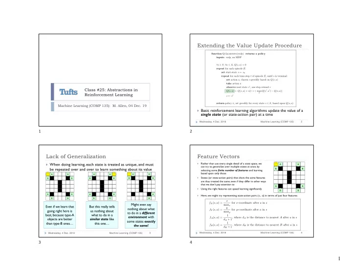
Extending the Value Update Procedure function Q-Learning ( mdp ) returns a policy inputs : mdp , an MDP ∀ s ∈ S, ∀ a ∈ A, Q ( s, a ) = 0 repeat for each episode E : set start-state s ← s 0 repeat for each time-step t of episode E , until s is terminal: set action a , chosen ✏ -greedily based on Q ( s, a ) take action a observe next state s 0 , one-step reward r Class #25: Abstractions in a 0 Q ( s 0 , a 0 ) − Q ( s, a )] Q ( s, a ) ← Q ( s, a ) + ↵ [ r + � max Reinforcement Learning s ← s 0 return policy ⇡ , set greedily for every state s ∈ S , based upon Q ( s, a ) Machine Learning (COMP 135): M. Allen, 04 Dec. 19 } Basic reinforcement learning algorithms update the value of a single state (or state-action pair) at a time 2 Wednesday, 4 Dec. 2019 Machine Learning (COMP 135) 1 2 Lack of Generalization Feature Vectors Rather than use every single detail of a state space, we } When doing learning, each state is treated as unique, and must } A A can try to generalize over multiple states at once, by be repeated over and over to learn something about its value B B selecting some finite number of features and learning based upon only those A A A A A A States (or state-action pairs) that share the same features } B B B B B B are thus treated the same, even if they differ in other ways that we don’t pay attention to A A Using the right features can speed learning significantly } B B A A A A A Here, we might try representing state-action pairs ( s , a ) in terms of just four features: } B B B B B x f X ( s, a ) = for x -coordinate after a in s Might even say max x Even if we learn that But this really tells y nothing about what f Y ( s, a ) = for y -coordinate after a in s going right here is us nothing about max y to do in a different best, because type-A what to do in a 1 environment with f A ( s, a ) = d A + 1, where d A is the distance to nearest A after a in s objects are better similar state like some states exactly than type-B ones… this one… 1 the same! f B ( s, a ) = d B + 1, where d B is the distance to nearest B after a in s 4 Wednesday, 4 Dec. 2019 Machine Learning (COMP 135) 3 Wednesday, 4 Dec. 2019 Machine Learning (COMP 135) 3 4 1

Choosing Feature Vectors Value Functions over Features } We want to choose values that seem to be } One issue is that when we use simpler features, we don’t A A important to problem success B B always know which ones to use } When we represent them, it has been shown that we get better results if we } States may share features and still have very different values normalize features, ensuring that each is in same, unit range: } Some features may turn out to be more or less important A A 0 ≤ f i ( s, a ) ≤ 1 } We want to learn a proper function that tells us how much we B B should pay attention to each feature x } We may assume this function is linear f X ( s, a ) = for x -coordinate after a in s max x } This means that the value of a state is a simple combination of y f Y ( s, a ) = for y -coordinate after a in s weights applied to each feature max y 1 } While this assumption may not be the right one in some f A ( s, a ) = d A + 1, where d A is the distance to nearest A after a in s domains, it can often be the basis of a good approximation 1 f B ( s, a ) = d B + 1, where d B is the distance to nearest B after a in s 6 Wednesday, 4 Dec. 2019 Machine Learning (COMP 135) 5 Wednesday, 4 Dec. 2019 Machine Learning (COMP 135) 5 6 Linear Functions over Features Setting the Weights Initially, we may not know which features really matter } } What we want is to learn the set of weights needed to In some cases, we may have knowledge that tells us some are more important than others, } and we will weight them more properly calculate our U - or Q -values In other cases, we may treat them all the same } For instance, in our grid problem, we might start with all weights the same ( 1.0 ) } U ( s ) = w 1 f 1 ( s ) + w 2 f 2 ( s ) + · · · + w n f n ( s ) After Right, at ( x,y ) = (2,1), Q ( s, Right ) = w X f X ( s, a ) + w Y f Y ( s, a ) + w A f A ( s, a ) + w B f B ( s, a ) distance 0 to A, distance 2 to B = (1 . 0 × 2 / 7) + (1 . 0 × 1 / 7) + (1 . 0 × 1) + (1 . 0 × 1 / 3) Q ( s, a ) = w 1 f 1 ( s, a ) + w 2 f 2 ( s, a ) + · · · + w n f n ( s, a ) = 1 . 76 A A B B Q ( s, Down ) = w X f X ( s, a ) + w Y f Y ( s, a ) + w A f A ( s, a ) + w B f B ( s, a ) = (1 . 0 × 1 / 7) + (1 . 0 × 2 / 7) + (1 . 0 × 1 / 3) + (1 . 0 × 1) } For instance, for our grid problem: = 1 . 76 Q ( s, a ) = w X f X ( s, a ) + w Y f Y ( s, a ) + w A f A ( s, a ) + w B f B ( s, a ) Initially, many states may end up with identical value estimates. If it A A turned out that position didn’t matter, and both A- and B-type objects B B were equally valuable, this would be fine. Typically, however, this is not the case, and we will need to adjust our weights dynamically as we go. 8 Wednesday, 4 Dec. 2019 Machine Learning (COMP 135) 7 Wednesday, 4 Dec. 2019 Machine Learning (COMP 135) 7 8 2

Adjusting the Weights Q-Learning with Function Approximation Now, when we take an action, we adjust weight-values and then compute Q - values } In normal Q-learning, we evaluate a state-action pair ( s,a ) based on } For example: we take the R IGHT action and get a large positive reward, which } the results we get ( r and s ′ ) and update the single pair value : means we could increase weights on contributing features δ = r + γ max Q ( s 0 , a 0 ) − Q ( s, a ) δ = r + γ max Q ( s 0 , a 0 ) − Q ( s, Right) = 10 a 0 a 0 Q ( s, a ) ← Q ( s, a ) + α δ w X ← w X + α δ f X ( s, a ) ← 1 . 0 + 0 . 9 × 10 × 2 / 7 = 3 . 57 A A B B w Y ← w Y + α δ f Y ( s, a ) } Now, we will instead update each of the weights on our features ← 1 . 0 + 0 . 9 × 10 × 1 / 7 = 2 . 29 } If outcomes are particularly good or bad, we change weights accordingly w A ← w A + α δ f A ( s, a ) } This affects all (state, action) pairs that share features with current one ← 1 . 0 + 0 . 9 × 10 × 1 = 10 . 0 A A w B ← w B + α δ f B ( s, a ) Q ( s 0 , a 0 ) − Q ( s, a ) δ = r + γ max B B ← 1 . 0 + 0 . 9 × 10 × 1 / 3 = 4 . 0 a 0 Q ( s, Right ) = (3 . 57 × 2 / 7) + (2 . 29 × 1 / 7) + (10 . 0 × 1) + (4 . 0 × 1 / 3) ∀ i, w i ← w i + α δ f i ( s, a ) = 12 . 69 10 Wednesday, 4 Dec. 2019 Machine Learning (COMP 135) 9 Wednesday, 4 Dec. 2019 Machine Learning (COMP 135) 9 10 Adjusting the Weights Adjusting the Weights Later, if we take the D OWN action from the same state, and get a large negative Note: since we adjust the weights that are used to calculate the Q -values of any } } cost-value, we might down-grade weights on the contributing features (state, action) pairs, what happens when we encounter one new outcome actually affects the Q -value of all the pairs at once We are thus potentially learning a value function over our entire space , even } δ = r + γ max Q ( s 0 , a 0 ) − Q ( s, Down ) = − 20 though it is based only on a single outcome at a time, which can speed up learning a 0 w X ← w X + α δ f X ( s, a ) ← 3 . 57 + 0 . 9 × − 20 × 1 / 7 = 1 . 0 A A w Y ← w Y + α δ f Y ( s, a ) B B Q ( s 0 , a 0 ) − Q ( s, Down ) = − 20 δ = r + γ max ← 2 . 29 + 0 . 9 × − 20 × 2 / 7 = − 2 . 85 After Down, we have a 0 changed weights, which w A ← w A + α δ f A ( s, a ) changes the Q -value of Q ( s, Down ) = (1 . 0 × 1 / 7) + ( − 2 . 85 × 2 / 7) + (4 . 0 × 1 / 3) + ( − 14 . 0 × 1) not only one state-action ← 10 . 0 + 0 . 9 × − 20 × 1 / 3 = 4 . 0 = − 13 . 34 pair, but all of them . w B ← w B + α δ f B ( s, a ) A A Here, we see the updated Q ( s, Right ) = (1 . 0 × 2 / 7) + ( − 2 . 85 × 1 / 7) + (4 . 0 × 1) + ( − 14 . 0 × 1 / 3) ← 4 . 0 + 0 . 9 × − 20 × 1 = − 14 . 0 value for going Right B B = − 0 . 79 (this was 12.69 before). Q ( s, Down ) = (1 . 0 × 1 / 7) + ( − 2 . 85 × 2 / 7) + (4 . 0 × 1 / 3) + ( − 14 . 0 × 1) = − 13 . 34 12 Wednesday, 4 Dec. 2019 Machine Learning (COMP 135) 11 Wednesday, 4 Dec. 2019 Machine Learning (COMP 135) 11 12 3