U ( s ) = U ( s ) + [ r + U ( s 0 ) U ( s )] inputs : mdp , an - - PowerPoint PPT Presentation

u s u s r u s 0 u s
SMART_READER_LITE
LIVE PREVIEW

U ( s ) = U ( s ) + [ r + U ( s 0 ) U ( s )] inputs : mdp , an - - PowerPoint PPT Presentation

Learning the Value of a Policy } The dynamic programming algorithm we have seen works fine if we already know everything about an MDP system, including: Probabilities of all state-action transitions 1. Rewards we get in each case 2. } If we


slide-1
SLIDE 1

1

Class #25: Reinforcement Learning

Machine Learning (COMP 135): M. Allen, 22 Apr. 20

1

Learning the Value of a Policy

} The dynamic programming algorithm we have seen works

fine if we already know everything about an MDP system, including:

1.

Probabilities of all state-action transitions

2.

Rewards we get in each case

} If we don’t have this information, how can we figure out

the value of a policy?

} Turns out we can use a sampling method } “Follow the policy, and see what happens”

2 Monday, 20 Apr. 2020 Machine Learning (COMP 135)

2

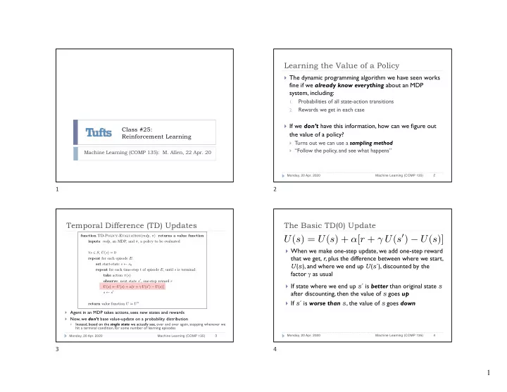
Temporal Difference (TD) Updates

} Agent in an MDP takes actions, sees new states and rewards } Now, we don’t base value-update on a probability distribution

}

Instead, based on the single state we actually see, over and over again, stopping whenever we hit a terminal condition, for some number of learning episodes

3 Monday, 20 Apr. 2020 Machine Learning (COMP 135)

function TD-Policy-Evaluation(mdp, π) returns a value function inputs: mdp, an MDP, and π, a policy to be evaluated ∀s ∈ S, U(s) = 0 repeat for each episode E: set start-state s ← s0 repeat for each time-step t of episode E, until s is terminal: take action π(s)

  • bserve: next state s0, one-step reward r

U(s) ← U(s) + α[r + γ U(s0) − U(s)] s ← s0 return value function U ≈ U π

3

The Basic TD(0) Update

} When we make one-step update, we add one-step reward

that we get, r, plus the difference between where we start, U(s), and where we end up U(s´), discounted by the factor g as usual

} If state where we end up s´ is better than original state s

after discounting, then the value of s goes up

} If s´ is worse than s, the value of s goes down

4 Monday, 20 Apr. 2020 Machine Learning (COMP 135)

U(s) = U(s) + α[r + γ U(s0) − U(s)]

4

slide-2
SLIDE 2

2 The Basic TD(0) Update

} We also weight the value-update amount by another

constant a, (less than 1), called a step-size parameter

1.

If this value shrinks to 0 over time, values stop changing

2.

If we do this slowly, the update will eventually converge to actual value of state if we follow the policy p

} For example, if we update over episodes, e = 1, 2, 3,…, we

can set the parameter for each episode to be:

5 Monday, 20 Apr. 2020 Machine Learning (COMP 135)

αe = 1 e U(s) = U(s) + α[r + γ U(s0) − U(s)]

5

Advantages and a Problem

} With TD updates, we only update the states we actually

see given the policy we are following

} Don’t need to know MDP dynamics } May only have to update very few states, saving much time to

get the values of those we actually reach under our policy

} However, this can be a source of difficulty: we may not be

able to find a better policy, since we don’t know values of states that we never happen to visit

6 Monday, 20 Apr. 2020 Machine Learning (COMP 135)

6

Exploration and Exploitation

} If we use the Dynamic Programming method, we calculate

the value of every state

} Easy to update policy (just be greedy) } This is exploitation: use best values seen to choose actions

} When we are learning, however, we sometimes don’t

know what certain states are like, because we’ve never actually seen them yet

} Our current policy may never get us to things we really want } Thus, we must use exploration: try out things even if our

current best policy doesn’t think it’s a good idea

7 Monday, 20 Apr. 2020 Machine Learning (COMP 135)

7

Almost-Greedy Policies

} One simple way to add exploration is to use a policy

that is mostly greedy, but not always

} An “epsilon-greedy” (e-greedy) policy sets some

probability threshold, e, and chooses actions by:

  • 1. Picking a random number R ∈ [0,1]
  • 2. If R ≤ e, choosing the action at random
  • 3. If R > e, acting in a greedy fashion (as before)

8 Monday, 20 Apr. 2020 Machine Learning (COMP 135)

8

slide-3
SLIDE 3

3 Learning with e-greedy policies

} We can add this idea to our sampling update method } After we take an action, and see a state-transition from s

to s´, we do the same updates as before:

} When we choose actions, we do so in an e-greedy way,

sometimes following the policy based on learned values, and sometimes trying random things

} Over enough time, this can converge to true value

function U* of the optimal policy p*

9 Monday, 20 Apr. 2020 Machine Learning (COMP 135)

U(s) = U(s) + α[r + γ U(s0) − U(s)]

9

TD-Learning

} Algorithm is the same, but explores using sometimes-greedy and

sometimes-probabilistic action-choices instead of fixed policy p

} We reduce learning parameter a just as before to converge

Monday, 20 Apr. 2020 Machine Learning (COMP 135) 10

function TD-Learning(mdp) returns a policy inputs: mdp, an MDP ∀s ∈ S, U(s) = 0 repeat for each episode E: set start-state s ← s0 repeat for each time-step t of episode E, until s is terminal: choose action a, using ✏-greedy policy based on U(s)

  • bserve next state s0, one-step reward r

U(s) ← U(s) + ↵[r + U(s0) − U(s)] s ← s0 return policy ⇡, set greedily for every state s ∈ S, based upon U(s)

10

Randomness and Weighting in Learning

} Our algorithm uses two parameters, a and e (plus the

usual discount factor g), to control its overall behavior

} Each can be adapted over time to control algorithm 1.

e: the amount of randomness in the policy

}

When we don’t know much, set it to a high value, so that we start off with lots of random exploration

}

We reduce this value over time until e = 0, and we are being purely greedy, and just exploiting what he have learned

2.

a: the weight on each learning-update step

}

Reduce this over time, as well: when a = 0, U-values don’t change anymore, and we can converge on final policy values

Monday, 20 Apr. 2020 Machine Learning (COMP 135) 11

11

Randomness and Weighting in Learning

} The control parameters a and e give us simple ways to

control complex learning behavior

} We don’t always want to reduce each over time } In a purely stationary environment, where system

dynamics don’t ever change, and all probabilities stay the same, we can simply slowly reduce each until we converge upon a stable learned behavior

} In a non-stationary environment, where things may

change at some point, learned solutions may quit working

Monday, 20 Apr. 2020 Machine Learning (COMP 135) 12

12

slide-4
SLIDE 4

4 Non-Stationary Environments

} Suppose environment starts off in one configuration: } Over time, we can learn a policy for shortest path to goal } By letting e and a go to 0, the policy becomes stable

Monday, 20 Apr. 2020 Machine Learning (COMP 135) 13

GOAL s0

13

Non-Stationary Environments

} The environment may change, however: } If e and a stay at 0, policy is sub-optimal from now on

Monday, 20 Apr. 2020 Machine Learning (COMP 135) 14

GOAL s0

14

Non-Stationary Environments

} We may be able to tell that environment changes, however } If value drops off over a long time, we can increase e and a

again, to resume learning and find new optimal policy

Monday, 20 Apr. 2020 Machine Learning (COMP 135) 15

GOAL s0

X X X X X X X X X X X X X X

15

Bellman Equations for Q-values

} Instead of the value of a state U(s), we can calculate the

value of a state-action pair Q(s,a)

} The value of taking action a in state s, and then following

the policy π after that:

} Similarly, we calculate optimal values Q*(s,a) of taking a

in state s, then following best possible policy after that:

} We can do learning for Q-values, too…

Monday, 20 Apr. 2020 Machine Learning (COMP 135) 16

Qπ(s, a) =

  • s

P(s, a, s) [R(s, a, s) + γ Qπ(s, π(s))] Q(s, a) =

  • s

P(s, a, s) ⇥ R(s, a, s) + γ max

a

Q(s, a) ⇤ 16

slide-5
SLIDE 5

5 TD (SARSA) Learning for Q-values

} Same basic RL method, converging to optimal Q* } Called SARSA, due to information used (s, a, r, s´, a´)

Monday, 20 Apr. 2020 Machine Learning (COMP 135) 17

function SARSA-Learning(mdp) returns a policy inputs: mdp, an MDP ∀s ∈ S, ∀a ∈ A, Q(s, a) = 0 repeat for each episode E: set start-state s ← s0 set action a, chosen ✏-greedily based on Q(s, a) repeat for each time-step t of episode E, until s is terminal: take action a

  • bserve next state s0, one-step reward r

set next action a0, chosen ✏-greedily based on Q(s0, a0) Q(s, a) ← Q(s, a) + ↵[r + Q(s0, a0) − Q(s, a)] s ← s0; a ← a0 return policy ⇡, set greedily for every state s ∈ S, based upon Q(s, a)

17

On-Policy Updates

} Both basic TD and SARSA are on-policy learning/update methods } We choose our initial action (a) based on current e-greedy policy

Monday, 20 Apr. 2020 Machine Learning (COMP 135) 18

function SARSA-Learning(mdp) returns a policy inputs: mdp, an MDP ∀s ∈ S, ∀a ∈ A, Q(s, a) = 0 repeat for each episode E: set start-state s ← s0 set action a, chosen ✏-greedily based on Q(s, a) repeat for each time-step t of episode E, until s is terminal: take action a

  • bserve next state s0, one-step reward r

set next action a0, chosen ✏-greedily based on Q(s0, a0) Q(s, a) ← Q(s, a) + ↵[r + Q(s0, a0) − Q(s, a)] s ← s0; a ← a0 return policy ⇡, set greedily for every state s ∈ S, based upon Q(s, a)

18

On-Policy Updates

} When we do the value update, we also choose the next action (a´) based

  • n the same current e-greedy policy

Monday, 20 Apr. 2020 Machine Learning (COMP 135) 19

function SARSA-Learning(mdp) returns a policy inputs: mdp, an MDP ∀s ∈ S, ∀a ∈ A, Q(s, a) = 0 repeat for each episode E: set start-state s ← s0 set action a, chosen ✏-greedily based on Q(s, a) repeat for each time-step t of episode E, until s is terminal: take action a

  • bserve next state s0, one-step reward r

set next action a0, chosen ✏-greedily based on Q(s0, a0) Q(s, a) ← Q(s, a) + ↵[r + Q(s0, a0) − Q(s, a)] s ← s0; a ← a0 return policy ⇡, set greedily for every state s ∈ S, based upon Q(s, a)

19

The Effect of On-Policy Updates

} When we do this sort of updating, we are not basing our value

calculation on the best possible policy

} Instead, we are basing it on our learning policy, which means

the values that we base our updates and choices on will combine the values that we get from:

1.

greedy action selection for exploitation

2.

random actions in some states for exploration

} Values we learn can reflect what would happen in a state if we

sometimes acted in a non-optimal way

} For example, on the edge of a cliff, we will sometimes randomly

explore jumping off the cliff when learning

} Edge-states are thus risky, and get lower value than they would really

have under the optimal policy (where we only do the best thing, and never jump)

Monday, 20 Apr. 2020 Machine Learning (COMP 135) 20

20

slide-6
SLIDE 6

6 Off-Policy Methods

} One possible solution is to update the values we learn

based on the best actions only

} That is, we ignore rewards and outcomes that come from

any of the possible bad actions we take when exploring

} The policy being updated is then not the current learning

version, but the optimal one

} This is the policy that we wanted to learn in the end, anyway!

} How can we do this?

Monday, 20 Apr. 2020 Machine Learning (COMP 135) 21

21

Q-Learning: Off-Policy Updates

} We still choose actions (a ) in an e-greedy way (so we are sometimes random) } However, we update values based upon whatever action would actually be best

Monday, 20 Apr. 2020 Machine Learning (COMP 135) 22

function Q-Learning(mdp) returns a policy inputs: mdp, an MDP ∀s ∈ S, ∀a ∈ A, Q(s, a) = 0 repeat for each episode E: set start-state s ← s0 repeat for each time-step t of episode E, until s is terminal: set action a, chosen ✏-greedily based on Q(s, a) take action a

  • bserve next state s0, one-step reward r

Q(s, a) ← Q(s, a) + ↵[r + max

a0 Q(s0, a0) − Q(s, a)]

s ← s0 return policy ⇡, set greedily for every state s ∈ S, based upon Q(s, a)

22

Comparing the Methods: Cliff Problem

} Shortest path to the goal

goes along edge of a cliff

} SARSA learns safer path,

since edge-states get lower values due to random falls

} Q-Learning learns best

path, since it ignores random jumps off edge

} Why does QL do worse

in the end? How can we fix this over a period of time?

Monday, 20 Apr. 2020 Machine Learning (COMP 135) 23

Example from: Sutton & Barto, 1998

23

Unifying the Methods

} Both SARSA and Q-Learning can be made to converge to the

same optimal policy over time

} By reducing the epsilon-value in our e-greedy policy, we

eventually reduce the randomness

} Thus, the SARSA agent will eventually learn better values even

for risky states, and come to use the optimal policy, too (e.g. walking along the cliff’s edge)

} So what’s the difference?

} In many cases, Q-Learning can converge on values somewhat faster } Doesn’t have to spend time “fixing” the values of states where it has

  • ver-estimated negative risk

} Thus we can reduce the e-value more rapidly, and learn optimal

state-values more quickly

} What are the potential risks of doing this?

Monday, 20 Apr. 2020 Machine Learning (COMP 135) 24

24

slide-7
SLIDE 7

7 End of Semester

} T

  • pics: Reinforcement Learning, Wrap-Up

} Note: Last live Q&A this Wednesday (none next week) } Project 02: due Monday, 27 April, 5:00 PM

} Sentiment analysis in review text } Uses two different models of textual data

} Final Paper: due Friday, 08 May, 5:00 PM

} Prompt, rubric, and sample essay on Piazza now

} Office Hours:

} Hours and Zoom links can be found on Piazza and Canvas

Monday, 20 Apr. 2020 Machine Learning (COMP 135) 25

25