
SLIDE 1
Discrete Random Variables; Expectation 18.05 Spring 2014 Jeremy Orloff and Jonathan Bloom
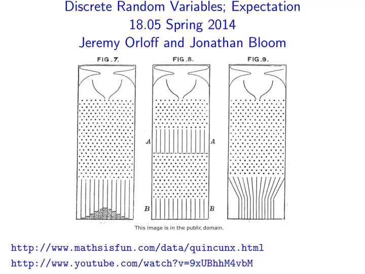
http://www.mathsisfun.com/data/quincunx.html http://www.youtube.com/watch?v=9xUBhhM4vbM
This image is in the public domain.
Discrete Random Variables; Expectation 18.05 Spring 2014 Jeremy - - PowerPoint PPT Presentation
Discrete Random Variables; Expectation 18.05 Spring 2014 Jeremy Orloff and Jonathan Bloom This image is in the public domain. http://www.mathsisfun.com/data/quincunx.html http://www.youtube.com/watch?v=9xUBhhM4vbM Board Question: Evil Squirrels One
This image is in the public domain.
May 27, 2014 2 / 28
May 27, 2014 3 / 28
1 The Randomizer holds the 6-sided die in one fist and
2 The Roller selects one of the Randomizer’s fists and
3 The Roller rolls the die in secret and reports the result
May 27, 2014 4 / 28
May 27, 2014 5 / 28
May 27, 2014 6 / 28
May 27, 2014 7 / 28
May 27, 2014 8 / 28
May 27, 2014 9 / 28
May 27, 2014 10 / 28
May 27, 2014 11 / 28
May 27, 2014 12 / 28
May 27, 2014 13 / 28
May 27, 2014 14 / 28
May 27, 2014 15 / 28
May 27, 2014 16 / 28
May 27, 2014 17 / 28
May 27, 2014 18 / 28
May 27, 2014 19 / 28
May 27, 2014 20 / 28
May 27, 2014 21 / 28
May 27, 2014 22 / 28
May 27, 2014 23 / 28
May 27, 2014 24 / 28
May 27, 2014 25 / 28
May 27, 2014 26 / 28
May 27, 2014 27 / 28
May 27, 2014 28 / 28