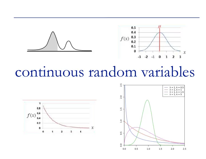
continuous random variables continuous random variables Discrete - - PowerPoint PPT Presentation

continuous random variables

continuous random variables Discrete random variable: takes values in a finite or countable set, e.g. X ∈ {1,2, ..., 6} with equal probability X is positive integer i with probability 2-i Continuous random variable: takes values in an uncountable set, e.g. X is the weight of a random person (a real number) X is a randomly selected point inside a unit square X is the waiting time until the next packet arrives at the server

!2

f(x): R→R, the probability density function (or simply “density”) pdf

!3

f(x)

Require: I.e., distribution is: f(x) ≥ 0, and nonnegative, and ∫ f(x) dx = 1 normalized, just like discrete PMF

• ∞

+∞

F(x): the cumulative distribution function (aka the “distribution”) F(a) = P(X ≤ a) = ∫ f(x) dx (Area left of a) P(a < X ≤ b) =

b

f(x)

a

a −∞

cdf

!4

F(x): the cumulative distribution function (aka the “distribution”) F(a) = P(X ≤ a) = ∫ f(x) dx (Area left of a) P(a < X ≤ b) = F(b) - F(a) (Area between a and b)

b

f(x)

a

a −∞

cdf

!5

F(x): the cumulative distribution function (aka the “distribution”) F(a) = P(X ≤ a) = ∫ f(x) dx (Area left of a) P(a < X ≤ b) = F(b) - F(a) (Area between a and b) Relationship between f(x) and F(x)?

b

f(x)

a

a −∞

cdf

!6

F(x): the cumulative distribution function (aka the “distribution”) F(a) = P(X ≤ a) = ∫ f(x) dx (Area left of a) P(a < X ≤ b) = F(b) - F(a) (Area between a and b) A key relationship:

b

f(x)

a

a −∞

cdf

!7

f(x) = F(x), since F(a) = ∫ f(x) dx,

a −∞ d dx

Densities are not probabilities; e.g. may be > 1 P(X = a) = limε→0 P(a-ε < X ≤ a) = F(a)-F(a) = 0 I.e., the probability that a continuous r.v. falls at a specified point is zero. But the probability that it falls near that point is proportional to the density:

why is it called a density?

!8

a-ε/2 a a+ε/2 f(x)

Densities are not probabilities; e.g. may be > 1 P(X = a) = limε→0 P(a-ε < X ≤ a) = F(a)-F(a) = 0 I.e., the probability that a continuous r.v. falls at a specified point is zero. But the probability that it falls near that point is proportional to the density: P(a - ε/2 < X ≤ a + ε/2) = F(a + ε/2) - F(a - ε/2) ≈ ε • f(a) I.e., in a large random sample, expect more samples where density is higher (hence the name “density”).

why is it called a density?

!9

a-ε/2 a a+ε/2 f(x)

Much of what we did with discrete r.v.s carries over almost unchanged, with Σx... replaced by ∫... dx E.g. For discrete r.v. X, E[X] = Σx xp(x) For continuous r.v. X, sums and integrals; expectation

!10

Much of what we did with discrete r.v.s carries over almost unchanged, with Σx... replaced by ∫... dx E.g. For discrete r.v. X, E[X] = Σx xp(x) For continuous r.v. X, Why?

(a) We define it that way (b) The probability that X falls “near” x, say within x±dx/2, is ≈f(x)dx, so the “average” X should be ≈ Σ xf(x)dx (summed

• ver grid points spaced dx apart on the real line) and the

limit of that as dx→0 is ∫xf(x)dx

sums and integrals; expectation

!11

continuous random variables: summary Continuous random variable X has density f(x), and

Linearity E[aX+b] = aE[X]+b E[X+Y] = E[X]+E[Y] Functions of a random variable E[g(X)] = ∫g(x)f(x)dx

Alternatively, let Y = g(X), find the density of Y, say fY, and directly compute E[Y] = ∫yfY(y)dy.

properties of expectation

!13

still true, just as for discrete just as for discrete, but w/integral

variance

!14

Definition is same as in the discrete case Var[X] = E[(X-μ)2] where μ = E[X] Identity still holds: Var[X] = E[X2] - (E[X])2 proof “same”

example Let What is F(x)? What is E(X)?

!15

• 1 0 1 2

1

• 1 0 1 2

1

F(x) f(x)

FGF

Q

IEE

I

X 2 I

F

X

xHx dx Sox

dx

Eat

z

E

x7uydx

Is

example Let

!16

• 1 0 1 2

1

• 1 0 1 2

1

F(x) f(x)

Van

x

to 425

example Let

!17

• 1 0 1 2

1

• 1 0 1 2

1

F(x) f(x)

0.0 0.5 1.0 1.5 0.0 0.5 1.0 1.5 2.0

The Uniform Density Function Uni(0.5,1.0)

x f(x)

uniform random variables X ~ Uni(α,β) is uniform in [α,β] 0.5 (α) 1.0 (β) 2.0

The Uniform Density Function Uni(0.5,1.0)

x f(x)

uniform random variables X ~ Uni(α,β) is uniform in [α,β]

if α≤a≤b≤β: Yes, you should review your basic calculus; e.g., these 2 integrals would be good practice.

waiting for “events”

Radioactive decay: How long until the next alpha particle? Customers: how long until the next customer/packet arrives at the checkout stand/server? Buses: How long until the next #71 bus arrives on the Ave?

Yes, they have a schedule, but given the vagaries of traffic, riders with-bikes-and-baby- carriages, etc., can they stick to it?

Assuming events are independent, happening at some fixed average rate of λ per unit time – the waiting time until the next event is exponentially distributed (next slide)

!20

interval

dt

gone

Probevent

Adt

exponential random variables X ~ Exp(λ)

• 1

1 2 3 4 0.0 0.5 1.0 1.5 2.0

The Exponential Density Function

x f(x)

λ = 2 λ = 1

Exponential witnparam

A

exponential random variables X ~ Exp(λ)

= 1-F(t)

Memorylessness: Assuming exp distr, if you’ve waited s minutes, prob of waiting t more is exactly same as s = 0

E

X

Tox a e

DX L

D

ax

Jae dx

e I t

Relation to Poisson


 Same process, different measures: Poisson: how many events in a fixed time; 
 Exponential: how long until the next event

!23

λ is avg # per unit time; 
 1/λ is mean wait