Chapter 2: Random Variables In this chapter we will cover: 1. - - PDF document

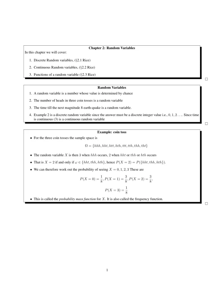
Chapter 2: Random Variables In this chapter we will cover:

• 1. Discrete Random variables, (§2.1 Rice)
• 2. Continuous Random variables, (§2.2 Rice)
• 3. Functions of a random variable (§2.3 Rice)

Random Variables

• 1. A random variable is a number whose value is determined by chance
• 2. The number of heads in three coin tosses is a random variable
• 3. The time till the next magnitude 8 earth-quake is a random variable.
• 4. Example 2 is a discrete random variable since the answer must be a discrete integer value i.e., 0, 1, 2 . . .. Since time

is continuous (3) is a continuous random variable Example: coin toss

• For the three coin tosses the sample space is

Ω = {hhh, hht, htt, hth, ttt, tth, thh, tht}

• The random variable X is then 3 when hhh occurs, 2 when hht or thh or hth occurs
• That is X = 2 if and only if ω ∈ {hht, thh, hth}, hence P(X = 2) = P({hht, thh, hth}).
• We can therefore work out the probability of seeing X = 0, 1, 2, 3 These are

P(X = 0) = 1 8, P(X = 1) = 3 8, P(X = 2) = 3 8, P(X = 3) = 1 8

• This is called the probability mass function for X. It is also called the frequency function.

1

Probability mass function

• A general discrete random variable which values x1, x2, x3, · · ·
• The probability mass function is

p(xi) = P(X = xi)

• From the rules of probability we must have that

0 ≤ p(xi) ≤ 1 and

• i

p(xi) = 1 Cumulative distribution function

• As an alternative to the mass function you can also defined the cumulative distribution function (cdf)
• Defined by

F(x) = P(X ≤ x)

1 2 3

• Prob. Mass Fn.

Probability 0.00 0.05 0.10 0.15 0.20 0.25 0.30 0.35 −1 1 2 3 4 0.0 0.2 0.4 0.6 0.8 1.0

Cumulative Distribution

x Probability

• 2

Cumulative distribution function

• Cumulative distribution functions are often denoted by capital letters e.g. F(x)
• Frequency functions by lowercase letters e.g. f(x)
• The CDF is non-decreasing and satisfies

lim

x→−∞ F(x) = 0, lim x→∞ F(x) = 1

Bernoulli Random variables

• 1. A Bernoulli random variable takes only two possible values 0 or 1
• 2. The probability it takes the value 1 is p, the probability it takes value 0 is 1 − p.
• 3. Its frequency function is

p(x) =    p if x = 1 1 − p if x = 0

• therwise
• 4. This can also be written as p(x) = px(1 − p)1−x for x = 0, 1 and 0 otherwise

Exercise Sketch the frequency and cdf for the random variable X where P(X = −1) = 1 10, P(X = 0) = 1 10, P(X = 1) = 3 10, P(X = 2) = 2 10, P(X = 3) = 0, P(X = 4) = 3 10 3

Exercise Whats the probability mass function for the cdf below?

2 4 6 8 10 0.0 0.2 0.4 0.6 0.8 1.0

Cumulative Distribution

x Probability

• Recommended Questions

From §2.5 of Rice you should do 1, 3, 5 (a), 7 Indicator random variables

• 1. If A is an event, then there is a probability p that the event happens, and 1 − p that is doesn’t happen
• 2. This can be coded as a random variable by taking the value 1 if it does happen and 0 if it does not.
• 3. Formally defined the indicator random variable IA(ω) by

IA(ω) = 1 ω ∈ A ω / ∈ A

• 4. Then IA(ω) is a Bernoulli r.v. for any A.

4

The Binomial distribution

• 1. Suppose that n independent experiments, each either ‘success’ or a ‘failure’, are run
• 2. Further suppose that for each experiment there is a fixed probability p of ‘success’
• 3. The number of successes in n experiments is called a binomial random variable
• 4. Its frequency function is

p(x) = n k

• pk(1 − p)n−k

for x ∈ {0, 1, · · · , n}. The Binomial distribution Some frequency functions when n = 10 for different values of p

• 2

4 6 8 10 0.0 0.1 0.2 0.3 0.4

p=0.1

x probability

• 2

4 6 8 10 0.00 0.10 0.20

p=0.3

x probability

• 2

4 6 8 10 0.00 0.10 0.20

p=0.5

x probability

• 2

4 6 8 10 0.0 0.1 0.2 0.3 0.4

p=0.9

x probability

The Binomial distribution

• 1. The mode is the x value with the highest probability. What is it in each of the cases shown above?
• 2. What is the relationship between the p = 0.1 and p = 0.9 case?

5

The Tay-Sachs disease

• Couples can be carriers of Tay-Sach disease
• Each child has a probability 0.25 of having the disease and this is independent across different children
• If the couple have 4 children, the number that will have the disease is Binomial (4, 0.25)
• These are P(k = 0) = 0.316, P(k = 1) = 0.422, P(k = 2) = 0.211, P(k = 3) = 0.047, P(k = 4) = 0.004

The Tay-Sachs disease

• What would these probabilities be if the probability of a single child having the disease is 0.5?
• What is the mode (i.e the most likely number)?

The geometric distribution

• The geometric distribution is also constructed from independent Bernoulli trials
• On each trial a ‘success’ occurs with probability p
• The geometric random variable counts the number of trials before the first success happens
• The frequency function is

p(k) = (1 − p)k−1p for k = 1, 2, 3, · · ·. 6

The geometric distribution Here are some numerical examples for different values of p.

• 5

10 15 0.0 0.2 0.4 0.6

p=0.1

x probability

• 5

10 15 0.0 0.2 0.4 0.6

p=0.3

x probability

• 5

10 15 0.0 0.2 0.4 0.6

p=0.5

x probability

• 5

10 15 0.0 0.2 0.4 0.6

p=0.6

x probability

Exercise

• 1. Which is more likely (i) 9 heads from 10 throws or (ii) 18 heads from 20 throws, of a fair coin
• 2. If X is a geometric random variable with p = 0.5 for what value of k is P(X ≤ K) ≈ 0.99

The hypergeometric distribution

• Suppose we have an urn with n balls, r black and n − r white.
• Let X be the number of black balls drawn when taking m balls without replacement. X has a hypergeometric

distribution.

• Its frequency function is

P(X = k) = r

k

n−r

m−k

• n

m

• Thus the probability of winning a lottery is hypergeometric

7

The Poisson distribution

• This has a frequency function

P(X = k) = λk k! exp(−λ) for k = 0, 1, 2, · · ·.

• This can be thought of as a limit of binomial trials as n gets large, and p is small, where λ = np.

The Poisson and binomial distributions Comparing numerically some Poisson and binomial distributions, the black is the Binomial, the red the Poisson.

• 1

2 3 4 5 0.0 0.2 0.4 0.6

n=5, p=0.1, lambda=0.5

x probability

• 2

4 6 8 10 0.00 0.10 0.20

n=5, p=0.1, lambda=0.5

x probability

• ● ● ● ●
• ● ● ● ●

5 10 15 20 0.00 0.05 0.10 0.15

n=20, p=0.5, lambda=10

x probability

• ● ● ●
• ●
• ● ● ●
• 20

40 60 80 100 0.00 0.04 0.08 0.12

n=100, p=0.1, lambda=10

x probability

• Examples
• Modelling the number of telephone calls coming into an exchange if the exchange has a large number of customers

which act more or less independently

• Modelling the number of α particles emitted from a radio active source
• Modelling the number of large accidents by an insurance company

8

Recommended questions From §2.5 Rice problems: 11,13,1,7,27,31,32. Continuous Random variables

• Suppose that the random variable of interest can take a continuum of values rather than lies in a discrete set
• In such a case the frequency function is replaced by the density function f(x), which is f(x) ≥ 0 and

∞

−∞

f(x)dx = 1

• If X is a random variable with density f(x) then

P(a < X < b) = b

a

f(x)dx Continuous Random variables

• For small δ, if f(x) is continuous then

P(x − δ 2 ≤ X ≤ x + δ 2) = x+ δ

2

x− δ

2

f(u)du ≈ δf(x)

• The cumulative distribution function F(x) is defined as

F(x) = P(X ≤ x) = x

−∞

f(u)du

• By calculus have that

f(x) = dF dx (x) Uniform Random Variables

• If X is uniformly distributed on the interval [a, b] then

f(x) =

• 1

b−a

a ≤ x ≤ b x < a or x > b

• The cumulative distribution function is

F(x) =    x < a

x−a b−a

a ≤ x ≤ b 1 x > b 9

Uniform Random Variables The density and cdf for the uniform on [0, 1].

−0.5 0.0 0.5 1.0 1.5 0.0 0.2 0.4 0.6 0.8 1.0

Uniform density

x Density −0.5 0.0 0.5 1.0 1.5 0.0 0.2 0.4 0.6 0.8 1.0

Uniform CDF

x Probability

The cdf

• By the properties of the cdf the inverse F −1(x) is well-defined.
• The pth quantile of F is defined to be xp such that F(xp) = p where p ∈ [0, 1]
• When p = 0.5 the quantile is called the median, when its 0.25 or 0.75 its called the lower or upper quartile of F.

10

Probabilities If X has a uniform [0, 1] distribution then P(X ∈ (0.5, 0.6)) is illustrated for both the density and cdf below

−0.5 0.0 0.5 1.0 1.5 0.0 0.2 0.4 0.6 0.8 1.0

Uniform density

x Density −0.5 0.0 0.5 1.0 1.5 0.0 0.2 0.4 0.6 0.8 1.0

Uniform CDF

x Probability

Exercise Sketch both the density and cdf function for a uniform [−1, 1] random variable and indicate what corresponds to the probability that x > 0. The exponential distribution

• The density function is

f(x) = λ exp(−λx) x ≥ 0 x < 0

• The cdf is

F(x) = 1 − exp(−λx) x ≥ 0 x < 0 11

‘Memoryless property’

• The exponential distribution is often used to model lifetimes or waiting times.
• It has the following property

P(T > t + s|T > s) = P(T > t), see page 49

• What does this mean?

The Normal distribution

• Probably the most used distribution in statistics is called the normal
• Its density function is given by

f(x) = 1 σ √ 2π exp

• −(x − µ)2

2σ2

• −∞ < x < ∞.
• The µ term is called the mean and the σ is called the standard deviation.
• The cdf does not have a nice formula, but Table 2 page A7 Rice gives numerical values for a standard normal

distribution. 12

The Normal distribution The plot shows three normal distributions. The black has µ = 0, σ = 1 (often called a standard normal). The red has µ = 5, σ = 1 while the blue has µ = 0, σ = 3.

−10 −5 5 10 0.0 0.1 0.2 0.3 0.4

Normal densities

x Density

13

The Normal distribution The figure shows the relationship between the shape of the normal density and the size of a standard deviation

−4 −2 2 4 0.0 0.1 0.2 0.3 0.4

Normal densitiy

Standard deviations from mean Density

Recommended Questions From §2.5 Rice look at questions 34, 40, 41, and 45. Also study the memoryless property of the exponential on page 49. Functions of a random variable

• Suppose X has a density function f(x), what is the density function of Y = g(X) for some function g?
• Since X is a random variable (i.e., its value its determined by chance), then g(X)’s value is also determined by

chance, hence it is also a random variable

• The function g(X) could be a linear function, i.e., Y = g(X) = aX + b
• Alternatively it could be a non-linear function Y = g(X) = X2.

14

Example Normal distribution

• Suppose X ∼ N(µ, σ2) (i.e. X has a normal distribution with mean µ and standard deviation σ) and that Y =

aX + b where a > 0.

• Consider the cdf for Y ,

FY (y) = P(Y ≤ y) = P(aX + b ≤ y) = P(X ≤ y − b a ) = FX(y − b a )

• Thus the density of Y is

fY (y) = d dy FX(y − b a ) = 1 afX(y − b a ) Example Normal distribution

• Thus

fY (y) = 1 aσ √ 2π exp

• −1

2 y − b − aµ aσ 2 so Y ∼ N(a + bµ, a2σ2) Example B page 59

• Let X ∼ N(µ, σ2), we want to find the probability that X is less than σ away from µ, i.e. P(|X − µ| < σ)
• This probability is

P(σ < X − µ < σ) = P(−1 < X − µ σ < 1)

• Using the previous result we see that Z = X−µ

σ

has a standard normal N(0, 1) distribution

• If Φ(x) is the cdf for the standard normal distribution, then we want

Φ(1) − Φ(−1) = 0.68 15

Example C page 59

• Find the density of X = Z2 where Z ∼ N(0, 1)
• We have

FX(x) = P(X ≤ x) = P(−√x ≤ Z ≤ √x) = Φ(√x) − Φ(−√x)

• Find the density of X by differentiating the cdf. Since Φ′(x) = φ(x) the density for the standard normal, we get

fX(z) = 1 2x−1/2φ(√x) + 1 2x−1/2φ(−√x) = φ(√x)

• More explicitly this is

fX(x) = x−1/2 √ 2π exp(−x/2). General rule

• Let X be a continuous variable with density f(x) and let Y = g(X) where g is differentiable, and monotonic
• The density of Y is

fY (y) = fX(g−1(y))

• d

dy g−1(y)

• Recommended Questions

From §2.5 Rice look at questions 53 (Hint use the results on a function of a random variable to convert the r.v. to a standard normal then use the tables at back of book), 55, 58, 59 and 67 (a, b) 16