SLIDE 8 normal random variables X is a normal random variable X ~ N(μ,σ2) Y = aX + b E[Y] = E[aX+b] = aμ + b Var[Y] = Var[aX+b] = a2σ2 normal random variables X is a normal random variable X ~ N(μ,σ2) Y = aX + b E[Y] = E[aX+b] = aμ + b Var[Y] = Var[aX+b] = a2σ2 Y ~ N(aμ + b, a2σ2) Important special case: Z = (X-μ)/σ ~ N(0,1)
E[ ], Var[ ] as expected;
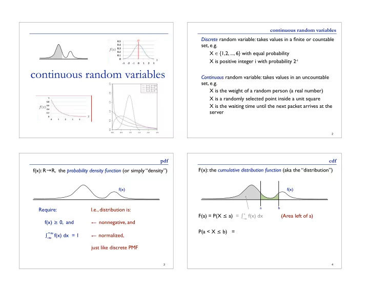
“normality” is the surprise
normal random variables X is a normal random variable X ~ N(μ,σ2) Y = aX + b E[Y] = E[aX+b] = aμ + b Var[Y] = Var[aX+b] = a2σ2 Y ~ N(aμ + b, a2σ2) Important special case: Z = (X-μ)/σ ~ N(0,1) Z ~ N(0,1) “standard (or unit) normal” Use Φ(z) to denote CDF, i.e. no closed form L
E[ ], Var[ ] as expected;
“normality” is the surprise
0.5000 0.4960 0.4920 0.4880 0.4840 0.4801 0.4761 0.4721 0.4681 0.0 0.5000 0.5040 0.5080 0.5120 0.5160 0.5199 0.5239 0.5279 0.5319 0.1 0.5398 0.5438 0.5478 0.5517 0.5557 0.5596 0.5636 0.5675 0.5714 0.2 0.5793 0.5832 0.5871 0.5910 0.5948 0.5987 0.6026 0.6064 0.6103 0.3 0.6179 0.6217 0.6255 0.6293 0.6331 0.6368 0.6406 0.6443 0.6480 0.4 0.6554 0.6591 0.6628 0.6664 0.6700 0.6736 0.6772 0.6808 0.6844 0.5 0.6915 0.6950 0.6985 0.7019 0.7054 0.7088 0.7123 0.7157 0.7190 0.6 0.7257 0.7291 0.7324 0.7357 0.7389 0.7422 0.7454 0.7486 0.7517 0.7 0.7580 0.7611 0.7642 0.7673 0.7704 0.7734 0.7764 0.7794 0.7823 0.8 0.7881 0.7910 0.7939 0.7967 0.7995 0.8023 0.8051 0.8078 0.8106 0.9 0.8159 0.8186 0.8212 0.8238 0.8264 0.8289 0.8315 0.8340 0.8365 1.0 0.8413 0.8438 0.8461 0.8485 0.8508 0.8531 0.8554 0.8577 0.8599 1.1 0.8643 0.8665 0.8686 0.8708 0.8729 0.8749 0.8770 0.8790 0.8810 1.2 0.8849 0.8869 0.8888 0.8907 0.8925 0.8944 0.8962 0.8980 0.8997 1.3 0.9032 0.9049 0.9066 0.9082 0.9099 0.9115 0.9131 0.9147 0.9162 1.4 0.9192 0.9207 0.9222 0.9236 0.9251 0.9265 0.9279 0.9292 0.9306 1.5 0.9332 0.9345 0.9357 0.9370 0.9382 0.9394 0.9406 0.9418 0.9429 1.6 0.9452 0.9463 0.9474 0.9484 0.9495 0.9505 0.9515 0.9525 0.9535 1.7 0.9554 0.9564 0.9573 0.9582 0.9591 0.9599 0.9608 0.9616 0.9625 1.8 0.9641 0.9649 0.9656 0.9664 0.9671 0.9678 0.9686 0.9693 0.9699 1.9 0.9713 0.9719 0.9726 0.9732 0.9738 0.9744 0.9750 0.9756 0.9761 2.0 0.9772 0.9778 0.9783 0.9788 0.9793 0.9798 0.9803 0.9808 0.9812 2.1 0.9821 0.9826 0.9830 0.9834 0.9838 0.9842 0.9846 0.9850 0.9854 2.2 0.9861 0.9864 0.9868 0.9871 0.9875 0.9878 0.9881 0.9884 0.9887 2.3 0.9893 0.9896 0.9898 0.9901 0.9904 0.9906 0.9909 0.9911 0.9913 2.4 0.9918 0.9920 0.9922 0.9925 0.9927 0.9929 0.9931 0.9932 0.9934
Φ(.46)
3.0 0.9987 0.9987 0.9987 0.9988 0.9988 0.9989 0.9989 0.9989 0.9990 3.1 0.9990 0.9991 0.9991 0.9991 0.9992 0.9992 0.9992 0.9992 0.9993 3.2 0.9993 0.9993 0.9994 0.9994 0.9994 0.9994 0.9994 0.9995 0.9995 3.3 0.9995 0.9995 0.9995 0.9996 0.9996 0.9996 0.9996 0.9996 0.9996 3.4 0.9997 0.9997 0.9997 0.9997 0.9997 0.9997 0.9997 0.9997 0.9997 z 0.00 0.01 0.02 0.03 0.04 0.05 0.06 0.07 0.08
1 2 3 0.0 0.1 0.2 0.3 0.4 0.5
The Standard Normal Density Function
x f(x)
µ = 0 σ = 1
Table of the Standard Normal Cumulative Distribution Function Φ(z)
E.g., see B&T p155, p531
μ±σ
NB: by symmetry
Φ(-z)=1-Φ(z)