4 Sums of Random Variables Many of the variables dealt with in - PDF document

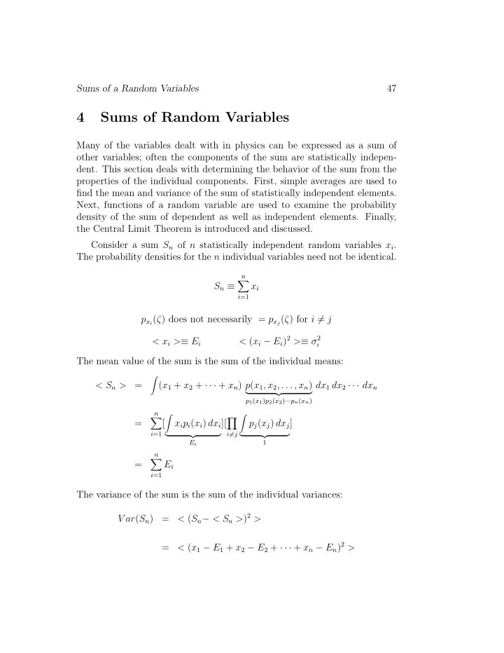
� � 47 Sums of a Random Variables 4 Sums of Random Variables Many of the variables dealt with in physics can be expressed as a sum of other variables; often the components of the sum are statistically indepen- dent. This section deals with determining the behavior of the sum from the properties of the individual components. First, simple averages are used to find the mean and variance of the sum of statistically independent elements. Next, functions of a random variable are used to examine the probability density of the sum of dependent as well as independent elements. Finally, the Central Limit Theorem is introduced and discussed. Consider a sum S n of n statistically independent random variables x i . The probability densities for the n individual variables need not be identical. n � S n ≡ x i i =1 p x i ( ζ ) does not necessarily = p x j ( ζ ) for i = j 2 2 < x i > ≡ E i < ( x i − E i ) > ≡ σ i The mean value of the sum is the sum of the individual means: � < S n > = ( x 1 + x 2 + · · · + x n ) p ( x 1 , x 2 , . . . , x n ) dx 1 dx 2 · · · dx n � �� � p 1 ( x 1 ) p 2 ( x 2 ) ··· p n ( x n ) n � � � � = [ x i p i ( x i ) dx i ][ p j ( x ) dx j ] j i =1 i = j � �� � � �� � E i 1 n � = E i i =1 The variance of the sum is the sum of the individual variances: < ( S n − < S n > ) 2 > V ar ( S n ) = < ( x 1 − E 1 + x 2 − E 2 + · · · + x n − E n ) 2 > =

� 48 Probability The right hand side of the above expression is a sum of terms, each quadratic in x , having the following form: < ( x i − E i )( x j − E j ) > = < x i x j > − < x i > E j − < x j > E i + E i E j = < x i x j > − E i E j � < x 2 2 2 i > − E i = σ i if i = j = 0 if i = j Therefore, n � σ 2 V ar ( S n ) = i . i =1 In the special case where all the individual x i ’s have the same probability density the above results reduce to 2 < S n > = nE i , V ar ( S n ) = nσ i . Physically, the width of p ( S n ) grows as √ n while the mean of S n grows as n . The probability density becomes more concentrated about the mean as n increases. If n is very large, the distribution develops a sharp narrow peak at the location of the mean. Now turn to the problem of finding the entire probability density, p S ( α ), for the sum of two arbitrary random variables x and y represented by the joint density p x,y ( ζ, η ). This is a straight forward application of functions of a random variable.

49 Sums of a Random Variables � ∞ � α − ζ P S ( α ) = dζ dη p x,y ( ζ, η ) −∞ −∞ d p s ( α ) = P S ( α ) dα � ∞ = dζ p x,y ( ζ, α − ζ ) −∞ In this expression p ( S ) is given as a single integral over the joint density p ( x, y ). The result is valid even when x and y are statistically dependent. The result simplifies somewhat when x and y are statistically independent, allowing the joint density to be factored into the product of two individual densities. � ∞ p S ( α ) = dζ p x ( ζ ) p y ( α − ζ ) if x and y are S.I. −∞ The integral operation involved in the last expression is known as convolu- tion . The probability density for the sum of two S.I. random variables is the convolution of the densities of the two individual variables. Convolu- tion appears in other disciplines as well. The transient output of a linear system (such as an electronic circuit) is the convolution of the impulse re- sponse of the system and the input pulse shape. The recorded output of a linear spectrometer (such as a grating spectrograph) is the convolution of the instrumental profile and the intrinsic spectrum being measured. The convolution of two functions p ( x ) and q ( x ) is designated by ⊗ and is defined as � ∞ p ⊗ q ≡ p ( z ) q ( x − z ) dz. −∞ It is easy to show from this expression that convolution is commutative, that is, the result does not depend on which function is taken first: a ⊗ b = b ⊗ a. Convolution is also distributive, a ⊗ ( b + c ) = a ⊗ b + a ⊗ c,

50 Probability and associative, a ⊗ ( b ⊗ c ) = ( a ⊗ b ) ⊗ c. Perhaps the best way to visualize the convolution integral is in terms of a series of successive steps. 1. FLIP q ( z ) ABOUT THE ORIGIN OF ITS ARGUMENT TO FORM THE MIRROR IMAGE q ( − z ). 2. SHIFT q ( − z ) TO THE RIGHT BY AN AMOUNT x TO FORM q ( z + x ). − 3. MULTIPLY q ( x − z ) BY p ( z ). 4. INTEGRATE THE PRODUCT AND PLOT THE RESULT.

51 Sums of a Random Variables 5. REPEAT 2 THROUGH 4 FOR DIFFERENT VALUES OF x . If p ( z ) and q ( z ) are each represented by a single analytic function for all z one can work out the convolution integral mathematically with little thought given to the above graphic procedure. On the other hand, when the input functions are zero in some regions or are only piecewise continuous, then the graphic procedure is useful in setting the proper limits of integration. Example: Sum of Two Uniformly Distributed Variables Given x and y are two statistically independent random variables, uni- formly distributed in the regions | x | ≤ a and | y | ≤ b . Problem Find the probability density p ( S ) for the sum S = x + y . Solution The form of the integral will depend on the value of S . Three separate regions need to be considered. Assume as indicated above that b < a . 0 < S < a − b

52 Probability � S + b 1 1 1 p ( S ) = ( )( ) dx = 2 a 2 b 2 a S − b a − b < S < a + b � a 1 1 a + b − S p ( S ) = ( )( ) dx = S − b 2 a 2 b (2 a )(2 b ) a + b < S p ( S ) = 0 since there is no overlap The symmetry of the problem demands that the result be even in S . The final result is plotted below.

53 Sums of a Random Variables When the widths of the two probability densities are the same, the density for the sum becomes triangular. . . . . . . . . . . . . . . . . . . . . . . . . . . . . . . . . . . . . . Example: Classical Intensity of Unpolarized Light Given An unpolarized beam of thermal light can be viewed as two sta- tistically independent beams of equal average intensity, polarized at right angles to each other. The total intensity I T is the sum of the intensities of each of the two polarized components, I 1 and I 2 . Problem Find the probability density for I T using the result from a pre- vious example that 1 p ( I 1 ) = √ exp[ − I 1 / 2 α ] I 1 > 0 2 παI 1 = 0 I 1 < 0 where α = < I 1 > . Solution Since the light is thermal and unpolarized, the intensity in each of the two polarization directions has the same density: p I 1 ( ζ ) = p I 2 ( ζ ).

54 Probability I I I I I I I I I I I � ∞ p ( I T ) = p I 1 ( I 1 ) p I 2 ( I T − I 1 ) dI 1 −∞ � ⎛ ⎞ � I T � exp[ − I 1 / 2 α ] exp[ ( I T − − I 1 ) / 2 α ] ⎠ dI 1 √ 2 παI 1 = ⎝ � 0 2 πα ( I T − I 1 ) � I 1 T [ I 1 ( I T − I 1 )] − 1 / 2 dI 1 = exp[ I T / 2 α ] − 2 πα 0 � I T / 2 1 1 1 − x ) − 1 / 2 dx ( I 2 2 = exp[ − I T / 2 α ] using x ≡ I − I T 1 T 2 πα 4 2 − I T 2 / � �� � π 1 = exp[ − I T / 2 α ] I T ≥ 0 2 α = 0 I T < 0

55 Sums of a Random Variables I I . . . . . . . . . . . . . . . . . . . . . . . . . . . . . . . . . . . . . In the two examples just considered the variables being summed had probability densities of the same functional form, rectangles for instance. Certainly this will not always be the case; for example one might be interested in the sum of two variables, one having a uniform density and the other having a Gaussian density. Yet even when the input variables do have probability densities of identical form, the density of the sum will in general have a different functional form than that of the input variables. The two previous examples illustrate this point. There are three special cases, however, where the functional form of the density is preserved during the addition of statistically independent, similarly distributed variables. The sum of two Gaussian variables is Gaussian. This is shown in an example below. Simply knowing that the result is Gaussian, though, is enough to allow one to predict the parameters of the density. Recall that a Gaussian is completely specified by its mean and variance. The fact that the means and variances add when summing S.I. random variables means that the mean of the resultant Gaussian will be the sum of the input means and the variance of the sum will be the sum of the input variances. The sum of two S.I. Poisson random variables is also Poisson. Here again, knowing that the result is Poisson allows one to determine the parameters in the sum density. Recall that a Poisson density is completely specified by one number, the mean, and the mean of the sum is the sum of the means.