
SLIDE 1
Discrete Random Variables; Expectation 18.05 Spring 2014
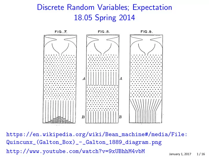
https://en.wikipedia.org/wiki/Bean_machine#/media/File: Quincunx_(Galton_Box)_-_Galton_1889_diagram.png http://www.youtube.com/watch?v=9xUBhhM4vbM
January 1, 2017 1 / 16
Discrete Random Variables; Expectation 18.05 Spring 2014 - - PowerPoint PPT Presentation
Discrete Random Variables; Expectation 18.05 Spring 2014 https://en.wikipedia.org/wiki/Bean_machine#/media/File: Quincunx_(Galton_Box)_-_Galton_1889_diagram.png http://www.youtube.com/watch?v=9xUBhhM4vbM January 1, 2017 1 / 16 Reading Review
January 1, 2017 1 / 16
January 1, 2017 2 / 16
January 1, 2017 3 / 16
January 1, 2017 4 / 16
January 1, 2017 5 / 16
January 1, 2017 6 / 16
January 1, 2017 7 / 16
January 1, 2017 8 / 16
January 1, 2017 9 / 16
January 1, 2017 10 / 16
January 1, 2017 11 / 16
January 1, 2017 12 / 16
January 1, 2017 13 / 16
January 1, 2017 14 / 16
January 1, 2017 15 / 16
MIT OpenCourseWare https://ocw.mit.edu
Spring 2014 For information about citing these materials or our Terms of Use, visit: https://ocw.mit.edu/terms.