
SLIDE 1
Measurement of CP Violation in Bs → J/ ψφ at CDF
Michal Kreps for the CDF collaboration
(rad)
s
β
- 1
1 )
- 1
(ps Γ ∆
- 0.6
- 0.4
- 0.2
0.0 0.2 0.4 0.6
- 1
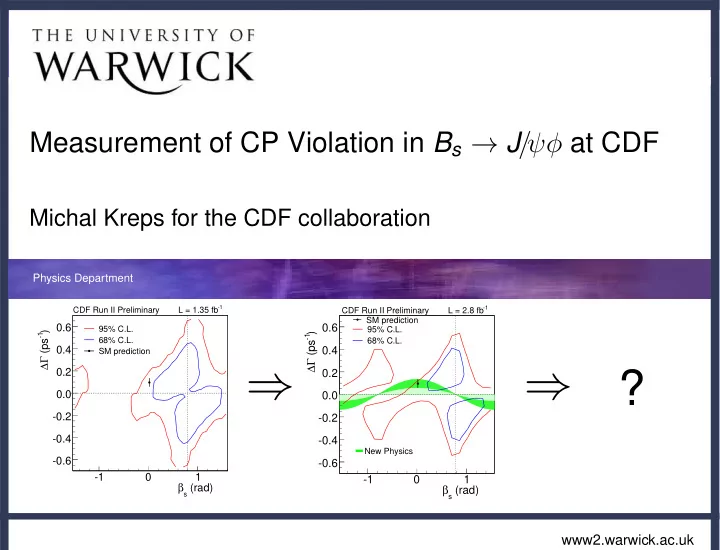
CDF Run II Preliminary L = 1.35 fb 95% C.L. 68% C.L. SM prediction
⇒
(rad)
s
β
- 1
1 )
- 1
(ps Γ ∆
- 0.6
- 0.4
- 0.2
0.0 0.2 0.4 0.6
- 1
CDF Run II Preliminary L = 2.8 fb 95% C.L. 68% C.L. SM prediction New Physics
⇒ ?
www2.warwick.ac.uk
Physics Department