more on expectation 1 2 properties of expectation properties of - - PowerPoint PPT Presentation

more on expectation
SMART_READER_LITE
LIVE PREVIEW

more on expectation 1 2 properties of expectation properties of - - PowerPoint PPT Presentation

properties of expectation Linearity of expectation, I For any constants a, b : E[ aX + b ] = a E[ X ] + b more on expectation 1 2 properties of expectation properties of expectation Linearity, II Note: Linearity is special! Let X


slide-1
SLIDE 1

more on expectation

1 2

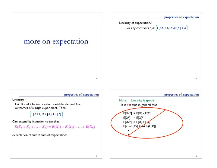
properties of expectation Linearity of expectation, I For any constants a, b: E[aX + b] = aE[X] + b

3

properties of expectation Linearity, II Let X and Y be two random variables derived from

  • utcomes of a single experiment. Then

Can extend by induction to say that expectation of sum = sum of expectations

E[X+Y] = E[X] + E[Y]

E(X1 + X2 + . . . + Xn) = E(X1) + E(X2) + . . . + E(Xn)

4

properties of expectation Note: Linearity is special! It is not true in general that E[X•Y] = E[X] • E[Y] E[X2] = E[X]2 E[X/Y] = E[X] / E[Y] E[asinh(X)] = asinh(E[X])

slide-2
SLIDE 2

variance

5 6

risk Alice & Bob are gambling. X = Alice’s gain per flip: E[X] = 0
 . . . Time passes . . .
 Alice (yawning) says “let’s raise the stakes” E[Y] = 0, as before. Are you (Bob) equally happy to play the new game? variance

7

E[X] measures the “average” or “central tendency” of X. What about its variability? variance

8

Definitions The variance of a random variable X with mean E[X] = μ is Var[X] = E[(X-μ)2],

  • ften denoted σ2.

The standard deviation of X is 
 σ = √Var[X]

slide-3
SLIDE 3

9

risk Alice & Bob are gambling (again). X = Alice’s gain per flip: E[X] = 0 Var[X] = 1 . . . Time passes . . . Alice (yawning) says “let’s raise the stakes” E[Y] = 0, as before. Var[Y] = 1,000,000 Are you (Bob) equally happy to play the new game? variance

10

Prob outcome X =============== 1/6 123 3 1/6 132 1 1/6 213 1 1/6 231 0 1/6 312 0 1/6 321 1 E(g(X)) = X

j∈Range(g(X))

jPr(g(X) = j)

= X

k∈Range(X)

g(k)Pr(X = k)

E(X) = X

k∈Range(X)

kPr(X = k)

The variance of a r.v. X with mean E[X] = μ is Var[X] = E[(X-μ)2],

  • ften denoted σ2.

what does variance tell us? The variance of a random variable X with mean E[X] = μ is Var[X] = E[(X-μ)2], often denoted σ2. 1: Square always ≥ 0, and exaggerated as X moves away 
 from μ, so Var[X] emphasizes deviation from the mean. II: Numbers vary a lot depending on exact distribution of X, but it is common that X is

within μ ± σ ~66% of the time, and within μ ± 2σ ~95% of the time.

(We’ll see the reasons for this soon.)

11

µ = 0 σ = 1

mean and variance μ = E[X] is about location; σ = √Var(X) is about spread

12

σ≈2.2 σ≈6.1 μ μ # heads in 20 flips, p=.5 # heads in 150 flips, p=.5 Blue arrows denote the interval μ ± σ
 (and note σ bigger in absolute terms in second ex., but smaller as a proportion of μ or max.)

slide-4
SLIDE 4

example Two games: a) flip 1 coin, win Y = $100 if heads, $-100 if tails b) flip 100 coins, win Z = (#(heads) - #(tails)) dollars Same expectation in both: E[Y] = E[Z] = 0 Same extremes in both: max gain = $100; max loss = $100 But 
 variability 
 is very 
 different:

σZ = 10 σY = 100

  • 100
  • 50

50 100 0.00 0.02 0.04 0.06 0.08 0.10 0.5 0.5

~ ~ ~ ~

horizontal arrows = μ ± σ


Var[aX+b] = a2 Var[X]

Ex: properties of variance

14

E[X] = 0 Var[X] = 1 Y = 1000 X E[Y] = E[1000 X] = 1000 E[X] = 0 Var[Y] = Var[103 X]=106Var[X] = 106

NOT linear; insensitive to location (b), quadratic in scale (a)

properties of variance

15

Var(X) = E[(X − µ)2] = E[X2 − 2µX + µ2] = E[X2] − 2µE[X] + µ2 = E[X2] − 2µ2 + µ2 = E[X2] − µ2 = E[X2] − (E[X])2

properties of variance

16

Example: What is Var[X] when X is outcome of one fair die? E[X] = 7/2, so

slide-5
SLIDE 5

In general: Var[X+Y] ≠ Var[X] + Var[Y]

Ex 1: Let X = ±1 based on 1 coin flip As shown above, E[X] = 0, Var[X] = 1 Let Y = -X; then Var[Y] = (-1)2Var[X] = 1 But X+Y = 0, always, so Var[X+Y] = 0 Ex 2: As another example, is Var[X+X] = 2Var[X]? properties of variance

17 ^^^^^^^

NOT linear

more variance examples

18

  • 4
  • 2

2 4 0.00 0.10

  • 4
  • 2

2 4 0.00 0.10

  • 4
  • 2

2 4 0.00 0.10

  • 4
  • 2

2 4 0.00 0.10 0.20

more variance examples

19

  • 4
  • 2

2 4 0.00 0.10

  • 4
  • 2

2 4 0.00 0.10

  • 4
  • 2

2 4 0.00 0.10

  • 4
  • 2

2 4 0.00 0.10 0.20

σ2 = 5.83 σ2 = 10 σ2 = 15 σ2 = 19.7