CS70: Jean Walrand: Lecture 36. Review: CDF and PDF. Expectation - - PowerPoint PPT Presentation

CS70: Jean Walrand: Lecture 36.

Continuous Probability 3

• 1. Review: CDF

, PDF

• 2. Review: Expectation
• 3. Review: Independence
• 4. Meeting at a Restaurant
• 5. Breaking a Stick
• 6. Maximum of Exponentials
• 7. Quantization Noise
• 8. Replacing Light Bulbs
• 9. Expected Squared Distance
• 10. Geometric and Exponential

Review: CDF and PDF.

Key idea: For a continuous RV, Pr[X = x] = 0 for all x ∈ ℜ. Examples: Uniform in [0,1]; throw a dart in a target. Thus, one cannot define Pr[outcome], then Pr[event]. Instead, one starts by defining Pr[event]. Thus, one defines Pr[X ∈ (−∞,x]] = Pr[X ≤ x] =: FX(x),x ∈ ℜ. Then, one defines fX(x) := d

dx FX(x).

Hence, fX(x)ε = Pr[X ∈ (x,x +ε)]. FX(·) is the cumulative distribution function (CDF) of X. fX(·) is the probability density function (PDF) of X.

Expectation

Definitions: (a) The expectation of a random variable X with pdf f(x) is defined as E[X] =

∞

−∞ xfX(x)dx.

(b) The expectation of a function of a random variable is defined as E[h(X)] =

∞

−∞ h(x)fX(x)dx.

(c) The expectation of a function of multiple random variables is defined as E[h(X)] =

• ···
• h(x)fX(x)dx1 ···dxn.

Justifications: Think of the discrete approximations of the continuous RVs.

Independent Continuous Random Variables

Definition: The continuous RVs X and Y are independent if Pr[X ∈ A,Y ∈ B] = Pr[X ∈ A]Pr[Y ∈ B],∀A,B. Theorem: The continuous RVs X and Y are independent if and only if fX,Y (x,y) = fX(x)fY (y). Proof: As in the discrete case. Definition: The continuous RVs X1,...,Xn are mutually independent if Pr[X1 ∈ A1,...,Xn ∈ An] = Pr[X1 ∈ A1]···Pr[Xn ∈ An],∀A1,...,An. Theorem: The continuous RVs X1,...,Xn are mutually independent if and only if fX(x1,...,xn) = fX1(x1)···fXn(xn). Proof: As in the discrete case.

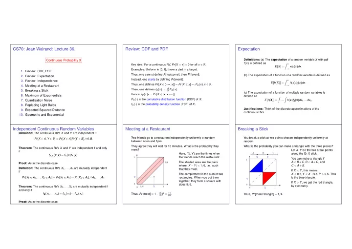
Meeting at a Restaurant

Two friends go to a restaurant independently uniformly at random between noon and 1pm. They agree they will wait for 10 minutes. What is the probability they meet? Here, (X,Y) are the times when the friends reach the restaurant. The shaded area are the pairs where |X −Y| < 1/6, i.e., such that they meet. The complement is the sum of two

• rectangles. When you put them

together, they form a square with sides 5/6. Thus, Pr[meet] = 1−( 5

6)2 = 11 36.

Breaking a Stick

You break a stick at two points chosen independently uniformly at random. What is the probability you can make a triangle with the three pieces? Let X,Y be the two break points along the [0,1] stick. You can make a triangle if A < B +C,B < A+C, and C < A+B. If X < Y, this means X < 0.5,Y < X +0.5,Y > 0.5. This is the blue triangle. If X > Y, we get the red triangle, by symmetry. Thus, Pr[make triangle] = 1/4.

Maximum of Two Exponentials

Let X = Expo(λ) and Y = Expo(µ) be independent. Define Z = max{X,Y}. Calculate E[Z]. We compute fZ, then integrate. One has Pr[Z < z] = Pr[X < z,Y < z] = Pr[X < z]Pr[Y < z] = (1−e−λz)(1−e−µz) = 1−e−λz −e−µz +e−(λ+µ)z Thus, fZ(z) = λe−λz + µe−µz −(λ + µ)e−(λ+µ)z,∀z > 0. Hence, E[Z] =

∞

0 zfZ(z)dz = 1

λ + 1 µ − 1 λ + µ .

Maximum of n i.i.d. Exponentials

Let X1,...,Xn be i.i.d. Expo(1). Define Z = max{X1,X2,...,Xn}. Calculate E[Z]. We use a recursion. The key idea is as follows: Z = min{X1,...,Xn}+V where V is the maximum of n −1 i.i.d. Expo(1). This follows from the memoryless property of the exponential. Let then An = E[Z]. We see that An = E[min{X1,...,Xn}]+An−1 = 1 n +An−1 because the minimum of Expo is Expo with the sum of the rates. Hence, E[Z] = An = 1+ 1 2 +···+ 1 n = H(n).

Quantization Noise

In digital video and audio, one represents a continuous value by a finite number of bits. This introduces an error perceived as noise: the quantization noise. What is the power of that noise? Model: X = U[0,1] is the continuous value. Y is the closest multiple

• f 2−n to X. Thus, we can represent Y with n bits. The error is

Z := X −Y. The power of the noise is E[Z 2]. Analysis: We see that Z is uniform in [0,a = 2−(n+1)]. Thus, E[Z 2] = a2 3 = 1 32−2(n+1). The power of the signal X is E[X 2] = 1

3.

Quantization Noise

We saw that E[Z 2] = 1

32−2(n+1) and E[X 2] = 1 3.

The signal to noise ratio (SNR) is the power of the signal divided by the power of the noise. Thus, SNR = 22(n+1). Expressed in decibels, one has SNR(dB) = 10log10(SNR) = 20(n +1)log10(2) ≈ 6(n +1). For instance, if n = 16, then SNR(dB) ≈ 112dB.

Replacing Light Bulbs

Say that light bulbs have i.i.d. Expo(1) lifetimes. We turn a light on, and replace it as soon as it burns out. How many light bulbs do we need to replace in t units of time? Theorem: The number Xt of replaced light bulbs is P(t). That is, Pr[Xt = n] = tn

n!e−t.

Proof: We see how Xt increases over the next ε ≪ 1 time units. Let A be the event that a burns out during [t,t +ε]. Then, Pr[Xt+ε = n] ≈ Pr[Xt = n,Ac]+Pr[Xt = n −1,A] = Pr[Xt = n]Pr[Ac]+Pr[Xt = n −1]Pr[A] ≈ Pr[Xt = n](1−ε)+Pr[Xt = n −1]ε. Hence, g(n,t) := Pr[Xt = n] is such that g(n,t +ε) ≈ g(n,t)−g(n,t)ε +g(n −1,t)ε.

Replacing Light Bulbs

Say that light bulbs have i.i.d. Expo(1) lifetimes. We turn a light on, and replace it as soon as it burns out. How many light bulbs do we need to replace in t units of time? Theorem: The number Xt of replaced light bulbs is P(t). That is, Pr[Xt = n] = tn

n!e−t.

Proof: (continued) We saw that g(n,t +ε) ≈ g(n,t)−g(n,t)ε +g(n −1,t)ε. Subtracting g(n,t), dividing by ε, and letting ε → 0, one gets g′(n,t) = −g(n,t)+g(n −1,t). You can check that these equations are solved by g(n,t) = tn

n!e−t.

Indeed, then g′(n,t) = tn−1 (n −1)!e−t −g(n,t) = g(n −1,t)−g(n,t).

Expected Squared Distance

Problem 1: Pick two points X and Y independently and uniformly at random in [0,1]. What is E[(X −Y)2]? Analysis: One has E[(X −Y)2] = E[X 2 +Y 2 −2XY] = 1 3 + 1 3 −21 2 1 2 = 2 3 − 1 2 = 1 6. Problem 2: What about in a unit square? Analysis: One has E[||X−Y||2] = E[(X1 −Y1)2]+E[(X2 −Y2)2] = 2× 1 6. Problem 3: What about in n dimensions? n

6.

Geometric and Exponential

The geometric and exponential distributions are similar. They are both memoryless. Consider flipping a coin every 1/N second with Pr[H] = p/N, where N ≫ 1. Let X be the time until the first H. Fact: X ≈ Expo(p). Analysis: Note that Pr[X > t] ≈ Pr[first Nt flips are tails] = (1− p N )Nt ≈ exp{−pt}. Indeed, (1− a

N )N ≈ exp{−a}.

Summary

Continuous Probability 3

◮ Continuous RVs are essentially the same as discrete RVs ◮ Think that X ≈ x with probability fX(x)ε ◮ Sums become integrals, .... ◮ The exponential distribution is magical: memoryless.