CS70: Jean Walrand: Lecture 27. Continuous Probability Normal - - PowerPoint PPT Presentation

CS70: Jean Walrand: Lecture 27.

CLT + Random Thoughts

• 1. Review: Continuous Probability
• 2. Normal Distribution
• 3. Central Limit Theorem
• 4. Random Thoughts

Continuous Probability

• 1. pdf: Pr[X ∈ (x,x +δ]] = fX(x)δ.
• 2. CDF: Pr[X ≤ x] = FX(x) =

x

−∞ fX(y)dy.

• 3. U[a,b], Expo(λ), target.
• 4. Expectation: E[X] =

∞

−∞ xfX(x)dx.

• 5. Expectation of function: E[h(X)] =

∞

−∞ h(x)fX(x)dx.

• 6. Variance: var[X] = E[(X −E[X])2] = E[X 2]−E[X]2.
• 7. Gaussian: N (µ,σ2) : fX(x) = ... “bell curve”

Normal Distribution.

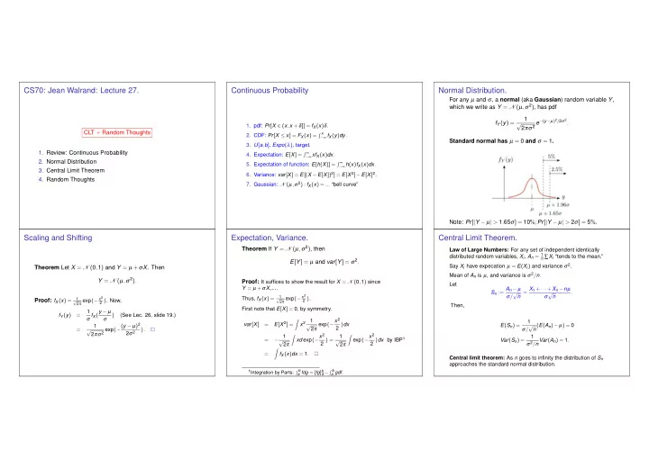
For any µ and σ, a normal (aka Gaussian) random variable Y, which we write as Y = N (µ,σ2), has pdf fY(y) = 1 √ 2πσ2 e−(y−µ)2/2σ2. Standard normal has µ = 0 and σ = 1. Note: Pr[|Y − µ| > 1.65σ] = 10%;Pr[|Y − µ| > 2σ] = 5%.

Scaling and Shifting

Theorem Let X = N (0,1) and Y = µ +σX. Then Y = N (µ,σ2). Proof: fX(x) =

1 √ 2π exp{− x2 2 }. Now,

fY (y) = 1 σ fX(y − µ σ ) (See Lec. 26, slide 19.) = 1 √ 2πσ2 exp{−(y − µ)2 2σ2 }.

Expectation, Variance.

Theorem If Y = N (µ,σ2), then E[Y] = µ and var[Y] = σ2. Proof: It suffices to show the result for X = N (0,1) since

Y = µ +σX,.... Thus, fX(x) =

1 √ 2π exp{− x2 2 }.

First note that E[X] = 0, by symmetry. var[X] = E[X 2] =

• x2

1 √ 2π exp{−x2 2 }dx = − 1 √ 2π

• xd exp{−x2

2 } = 1 √ 2π

• exp{−x2

2 }dx by IBP1 =

• fX(x)dx = 1.

1Integration by Parts:

b

a fdg = [fg]b a −

b

a gdf.

Central Limit Theorem.

Law of Large Numbers: For any set of independent identically distributed random variables, Xi, An = 1

n ∑Xi “tends to the mean.”

Say Xi have expecation µ = E(Xi) and variance σ2. Mean of An is µ, and variance is σ2/n. Let Sn := An − µ σ/√n = X1 +···+Xn −nµ σ√n . Then, E(Sn) = 1 σ/√n(E(An)− µ) = 0 Var(Sn) = 1 σ2/nVar(An) = 1. Central limit theorem: As n goes to infinity the distribution of Sn approaches the standard normal distribution.

Central Limit Theorem

Central Limit Theorem Let X1,X2,... be i.i.d. with E[X1] = µ and var(X1) = σ2. Define Sn := An − µ σ/√n = X1 +···+Xn −nµ σ√n . Then, Sn → N (0,1),as n → ∞. That is, Pr[Sn ≤ α] → 1 √ 2π

α

−∞ e−x2/2dx.

Proof: See EE126.

CI for Mean

Let X1,X2,... be i.i.d. with mean µ and variance σ2. Let An = X1 +···+Xn n . The CLT states that An − µ σ/√n = X1 +···+Xn −nµ σ√n → N (0,1) as n → ∞. Thus, for n ≫ 1, one has Pr[−2 ≤ |An − µ σ/√n | ≤ 2] ≈ 95%. Equivalently, Pr[µ ∈ [An −2 σ √n,An +2 σ √n]] ≈ 95%. That is, [An −2 σ √n,An +2 σ √n] is a 95%−CI for µ.

CI for Mean

Let X1,X2,... be i.i.d. with mean µ and variance σ2. Let An = X1 +···+Xn n . The CLT states that X1 +···+Xn −nµ σ√n → N (0,1) as n → ∞. Also, [An −2 σ √n,An +2 σ √n] is a 95%−CI for µ. Recall: Using Chebyshev, we found that (see Lec. 22, slide 6) [An −4.5 σ √n,An +4.5 σ √n] is a 95%−CI for µ. Thus, the CLT provides a smaller confidence interval.

Coins and normal.

Let X1,X2,... be i.i.d. B(p). Thus, X1 +···+Xn = B(n,p). Here, µ = p and σ =

• p(1−p). CLT states that

X1 +···+Xn −np

• p(1−p)n

→ N (0,1).

Coins and normal.

Let X1,X2,... be i.i.d. B(p). Thus, X1 +···+Xn = B(n,p). Here, µ = p and σ =

• p(1−p). CLT states that

X1 +···+Xn −np

• p(1−p)n

→ N (0,1) and [An −2 σ √n,An +2 σ √n] is a 95%−CI for µ with An = (X1 +···+Xn)/n. Hence, [An −2 σ √n,An +2 σ √n] is a 95%−CI for p. Since σ ≤ 0.5, [An −20.5 √n,An +20.5 √n] is a 95%−CI for p. Thus, [An − 1 √n,An + 1 √n] is a 95%−CI for p.

Summary

Gaussian and CLT

• 1. Gaussian: N (µ,σ2) : fX(x) = ... “bell curve”
• 2. CLT: Xn i.i.d. =

⇒ An−µ

σ/√n → N (0,1)

• 3. CI: [An −2 σ

√n,An +2 σ √n] = 95%-CI for µ.

Confusing Statistics: Simpson’s Paradox

The numbers are applications and admissions of males and females to the two colleges of a university. Overall, the admission rate of male students is 80% whereas it is only 51% for female students. A closer look shows that the admission rate is larger for female students in both colleges.... Female students happen to apply more to the college that admits fewer students.

More on Confusing Statistics

Statistics are often confusing:

◮ The average household annual income in the US is $72k.

Yes, but the median is $52k.

◮ The false alarm rate for prostate cancer is only 1%. Great,

but only 1 person in 8,000 has that cancer. So, there are 80 false alarms for each actual case.

◮ The Texas sharpshooter fallacy. Look at people living close

to power lines. You find clusters of cancers. You will also find such clusters when looking at people eating kale.

◮ False causation. Vaccines cause autism. Both vaccination

and autism rates increased....

◮ Beware of statistics reported in the media!

Choosing at Random: Bertrand’s Paradox

The figures corresponds to three ways of choosing a chord “at random.” The probability that the chord is larger than the side |AB| of an inscribed equilateral triangle is

◮ 1/3 if you choose a point A, then another point X uniformly at random

• n the circumference (left).

◮ 1/4 if you choose a point X uniformly at random in the circle and draw

the chord perpendicular to the radius that goes through X (center).

◮ 1/2 if you choose a point X uniformly at random on a given radius and

draw the chord perpendicular to the radius that goes through X (right).

Confirmation Bias

Confirmation bias is the tendency to search for, interpret, and recall information in a way that confirms one’s beliefs or hypotheses, while giving disproportionately less consideration to alternative possibilities. Confirmation biases contribute to overconfidence in personal beliefs and can maintain or strengthen beliefs in the face of contrary evidence. Three aspects:

◮ Biased search for information. E.g., ignoring articles that

dispute your beliefs.

◮ Biased interpretation. E.g., putting more weight on

confirmation than on contrary evidence.

◮ Biased memory. E.g., remembering facts that confirm your

beliefs and forgetting others.

Confirmation Bias: An experiment

There are two bags. One with 60% red balls and 40% blue balls; the other with the opposite fractions. One selects one of the two bags. As one draws balls one at time, one asks people to declare whether they think one draws from the first or second bag. Surprisingly, people tend to be reinforced in their original belief, even when the evidence accumulates against it.

Being Rational: ‘Thinking, Fast and Slow’

In this book, Daniel Kahneman discusses examples of our irrationality. Here are a few examples:

◮ A judge rolls a die in the morning. In the afternoon, he has to

sentence a criminal. Statistically, the sentence tends to be heavier if the outcome of the morning roll was high.

◮ People tend to be more convinced by articles printed in Times

Roman instead of Computer Modern Sans Serif.

◮ Perception illusions: Which horizontal line is longer?

It is difficult to think clearly!

What to Remember?

Professor, what should I remember about probability from this course? I mean, after the final. Here is what the prof. remembers:

◮ Given the uncertainty around us, we should understand some

probability.

◮ One key idea - what we learn from observations: the role of the

prior; Bayes’ rule; Estimation; confidence intervals... quantifying

• ur degree of certainty.

◮ This clear thinking invites us to question vague statements, and

to convert them into precise ideas.

Key Ideas in CS70 Probability

◮ Descriptive: Pr[A],E[X],E[h(X,Y)],πn,β(i),α(i) ◮ Inference: Pr[A|B],Pr[An|B],L[Y|X],E[Y|X],An ±2 σ √n ◮ Prescriptive: How to play a game, how to design, ....

What’s Next?

Professors, I loved this course so much! I want to learn more about discrete math and probability! Funny you should ask! How about

◮ CS170: Efficient Algorithms and Intractable Problems a.k.a.

Introduction to CS Theory: Graphs, Dynamic Programming, Complexity.

◮ EE126: Probability in EECS: An Application-Driven Course: PageRank,

Digital Links, Tracking, Speech Recognition, Planning, etc. Hands on labs with python experiments (GPS, Shazam, ...).

◮ CS188: Artificial Intelligence: Hidden Markov Chains, Bayes Networks,

Neural Networks.

◮ CS189: Introduction to Machine Learning: Regression, Neural

Networks, Learning, etc. Programming experiments with real-world applications.

◮ EE121: Digital Communication: Coding for communication and storage. ◮ EE223: Stochastic Control. ◮ EE229A: Information Theory; EE229B: Coding Theory.

Final Thoughts

More precisely: Some thoughts about the final .... How to study for the final?

◮ Lecture Slides; Notes; Discussion Problems; HW ◮ TA Office Hours, Prof. Office Hours, Reviews by TAs ◮ Next week: reviews during normal lecture hours:

◮ Discrete Math (Tuesday); ◮ Probability (Thursday).

Parting Thoughts

You have learned a lot in this course! Proofs, Graphs, Mod(p), RSA, Reed-Solomon, Decidability, Probability, ... , how to handle stress, how to sleep less, how to keep smiling, ... Difficult course? Yes! Useful? You bet! Finally, Thanks for taking the course! Thanks to the CS70 Staff:

◮ The Terrific Tutors ◮ The Rigorous Readers ◮ The Thrilling TAs ◮ The Amazing Assistants

See you on Tuesday.