
SLIDE 1
CS70: Jean Walrand: Lecture 26.
Continuous Probability
- 1. Examples
- 2. Events
- 3. Continuous Random Variables
- 4. Expectation
- 5. Bayes’ Rule
- 6. Multiple Random Variables
Continuous Probability - Pick a real number.
Choose a real number X, uniformly at random in [0,1000]. What is the probability that X is exactly equal to 100π = 314.1592625...? Well, ..., 0. Let [a,b] denote the event that the point X is in the interval [a,b]. Pr[[a,b]] = length of [a,b] length of [0,L] = b −a L = b −a 1000. Intervals like [a,b] ⊆ Ω = [0,L] are events. More generally, events in this space are unions of intervals. Example: the event A - “within 50 of 0 or 1000” is A = [0,50]∪[950,1000]. Thus, Pr[A] = Pr[[0,50]]+Pr[[950,10000]] = 1 10.
Continuous Probability - Pick a random real number.
Note: A radical change in approach. For a finite probability space, Ω = {1,2,...,N}, we started with Pr[ω] = pω. We then defined Pr[A] = ∑ω∈A pω for A ⊂ Ω. We used the same approach for countable Ω. For a continuous space, e.g., Ω = [0,L], we cannot start with Pr[ω], because this will typically be 0. Instead, we start with Pr[A] for some events A. Here, we started with A = interval, or union of intervals. Thus, the probability is a function from events to [0,1]. Can any function make sense? No! At least, it should be additive!. In our example, Pr[[0,50]∪[950,1000]] = Pr[[0,50]]+Pr[[950,1000]].
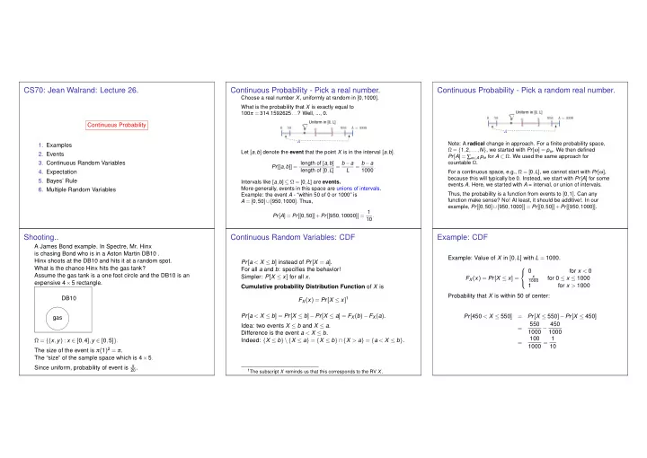
Shooting..
A James Bond example. In Spectre, Mr. Hinx is chasing Bond who is in a Aston Martin DB10 . Hinx shoots at the DB10 and hits it at a random spot. What is the chance Hinx hits the gas tank? Assume the gas tank is a one foot circle and the DB10 is an expensive 4×5 rectangle. DB10 gas Ω = {(x,y) : x ∈ [0,4],y ∈ [0,5]}. The size of the event is π(1)2 = π. The “size” of the sample space which is 4×5. Since uniform, probability of event is π
20.
Continuous Random Variables: CDF
Pr[a < X ≤ b] instead of Pr[X = a]. For all a and b: specifies the behavior! Simpler: P[X ≤ x] for all x. Cumulative probability Distribution Function of X is FX(x) = Pr[X ≤ x]1 Pr[a < X ≤ b] = Pr[X ≤ b]−Pr[X ≤ a] = FX(b)−FX(a). Idea: two events X ≤ b and X ≤ a. Difference is the event a < X ≤ b. Indeed: {X ≤ b}\{X ≤ a} = {X ≤ b}∩{X > a} = {a < X ≤ b}.
1The subscript X reminds us that this corresponds to the RV X.