[PPT] - Central Limit Theorem, Joint Distributions 18.05 Spring 2018 0.5 PowerPoint Presentation

SLIDE 1

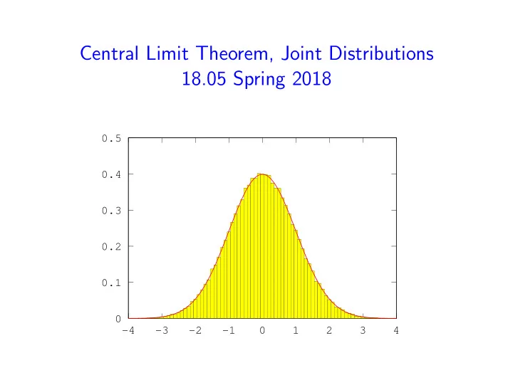
Central Limit Theorem, Joint Distributions 18.05 Spring 2018

0.1 0.2 0.3 0.4 0.5

4
3
2
1

1 2 3 4

SLIDE 2

Exam next Wednesday

Exam 1 on Wednesday March 7, regular room and time. Designed for 1 hour. You will have the full 80 minutes. Class on Monday will be review. Practice materials posted. Learn to use the standard normal table for the exam. No books or calculators. You may have one 4 × 6 notecard with any information you like.

February 27, 2018 2 / 31

SLIDE 3

The bell-shaped curve

−4 −2 2 4 0.1 0.2 0.3 0.4 0.5

z φ(z)

This is standard normal distribution N(0, 1): φ(z) = 1 √ 2π e−z2/2 N(0, 1) means that mean is µ = 0, and std deviation is σ = 1. Normal with mean µ, std deviation σ is N(µ, σ): φµ,σ(z) = 1 σ √ 2π e−(z−µ)2/2σ2

February 27, 2018 3 / 31

SLIDE 4

Lots of normal distributions

−4 −2 2 4 6 8 10 0.1 0.2 0.3 0.4 0.5 0.6 0.7 N(0, 1) N(4.5, 0.5) N(4.5, 2.25) N(6.5, 1.0) N(8.0, 0.5)

February 27, 2018 4 / 31

SLIDE 5

Standardization Random variable X with mean µ, standard deviation σ. Standardization: Y = X − µ σ . Y has mean 0 and standard deviation 1. Standardizing any normal random variable produces the standard normal. If X ≈ normal then standardized X ≈ stand. normal. We reserve Z to mean a standard normal random variable.

February 27, 2018 5 / 31

SLIDE 6

Board Question: Standardization

Here are the pdfs for four (binomial) random variables X. Standardize them, and make bar graphs of the standardized

distributions. Each bar should have area equal to the probability of

that value. (Each bar has width 1/σ, so each bar has height pdf·σ.) X n = 0 n = 1 n = 4 n = 9 1 1/2 1/16 1/512 1 1/2 4/16 9/512 2 6/16 36/512 3 4/16 84/512 4 1/16 126/512 5 126/512 6 84/512 7 36/512 8 9/512 9 1/512

February 27, 2018 6 / 31

SLIDE 7

Concept Question: Normal Distribution

X has normal distribution, standard deviation σ.

z −σ σ −2σ 2σ −3σ 3σ Normal PDF within 1 · σ ≈ 68% within 2 · σ ≈ 95% within 3 · σ ≈ 99% 68% 95% 99%

1. P(−σ < X < σ) is

(a) 0.025 (b) 0.16 (c) 0.68 (d) 0.84 (e) 0.95

2. P(X > 2σ)

(a) 0.025 (b) 0.16 (c) 0.68 (d) 0.84 (e) 0.95

answer: 1c, 2a

February 27, 2018 7 / 31

SLIDE 8

Central Limit Theorem

Setting: X1, X2, . . . i.i.d. with mean µ and standard dev. σ. For each n: X n = 1 n(X1 + X2 + . . . + Xn) average Sn = X1 + X2 + . . . + Xn sum. Conclusion: For large n: X n ≈ N

µ, σ2

n

Sn ≈ N
nµ, nσ2

Standardized

Sn or X n
≈ N(0, 1)

That is, Sn − nµ √nσ = X n − µ σ/√n ≈ N(0, 1).

February 27, 2018 8 / 31

SLIDE 9

CLT: pictures The standardized average of n i.i.d. Bernoulli(0.5) random variables with n = 1, 2, 12, 64.

0.05 0.1 0.15 0.2 0.25 0.3 0.35 0.4

3
2
1

1 2 3 0.05 0.1 0.15 0.2 0.25 0.3 0.35 0.4

3
2
1

1 2 3 0.05 0.1 0.15 0.2 0.25 0.3 0.35 0.4

3
2
1

1 2 3 0.05 0.1 0.15 0.2 0.25 0.3 0.35 0.4

4
3
2
1

1 2 3 4 February 27, 2018 9 / 31

SLIDE 10

CLT: pictures 2 Standardized average of n i.i.d. uniform random variables with n = 1, 2, 4, 12.

0.05 0.1 0.15 0.2 0.25 0.3 0.35 0.4

3
2
1

1 2 3 0.1 0.2 0.3 0.4 0.5

3
2
1

1 2 3 0.05 0.1 0.15 0.2 0.25 0.3 0.35 0.4

3
2
1

1 2 3 0.05 0.1 0.15 0.2 0.25 0.3 0.35 0.4

3
2
1

1 2 3 February 27, 2018 10 / 31

SLIDE 11

CLT: pictures 3 The standardized average of n i.i.d. exponential random variables with n = 1, 2, 8, 64.

0.2 0.4 0.6 0.8 1

3
2
1

1 2 3 0.1 0.2 0.3 0.4 0.5 0.6 0.7

3
2
1

1 2 3 0.1 0.2 0.3 0.4 0.5

3
2
1

1 2 3 0.1 0.2 0.3 0.4 0.5

3
2
1

1 2 3 February 27, 2018 11 / 31

SLIDE 12

CLT: pictures The non-standardized average of n Bernoulli(0.5) random variables, with n = 4, 12, 64. Spikier.

0.2 0.4 0.6 0.8 1 1.2 1.4

1
0.5

0.5 1 1.5 2 0.5 1 1.5 2 2.5 3

0.2

0.2 0.4 0.6 0.8 1 1.2 1.4 1 2 3 4 5 6 7

0.2

0.2 0.4 0.6 0.8 1 1.2 1.4 February 27, 2018 12 / 31

SLIDE 13

Table Question: Sampling from the standard normal distribution

As a table, produce two random samples from (an approximate) standard normal distribution. To make each sample, the table is allowed eight rolls of the 10-sided die. Note: µ = 5.5 and σ2 ≈ 8 for a single 10-sided die. Hint: CLT is about averages.

answer: The average of 9 rolls is a sample from the average of 9 independent random variables. The CLT says this average is approximately normal with µ = 5.5 and σ = 8.25/ √ 9 = 2.75 If x is the average of 9 rolls then standardizing we get z = x − 5.5 2.75 is (approximately) a sample from N(0, 1).

February 27, 2018 13 / 31

SLIDE 14

Board Question: CLT

1. Carefully write the statement of the central limit theorem.
2. To head the newly formed US Dept. of Statistics, suppose that

50% of the population supports Ani, 25% supports Ruthi, and the remaining 25% is split evenly between Efrat, Elan, David and Jerry. A poll asks 400 random people who they support. What is the probability that at least 55% of those polled prefer Ani?

3. What is the probability that less than 20% of those polled prefer

Ruthi?

answer: On next slide.

February 27, 2018 14 / 31

SLIDE 15

Solution

answer: 2. Let A be the fraction polled who support Ani. So A is the average of 400 Bernoulli(0.5) random variables. That is, let Xi = 1 if the ith person polled prefers Ani and 0 if not, so A = average of the Xi. The question asks for the probability A > 0.55. Each Xi has µ = 0.5 and σ2 = 0.25. So, E(A) = 0.5 and σ2

A = 0.25/400

r

σA = 1/40 = 0.025. Because A is the average of 400 Bernoulli(0.5) variables the CLT says it is approximately normal and standardizing gives A − 0.5 0.025 ≈ Z So P(A > 0.55) ≈ P(Z > 2) ≈ 0.025 Continued on next slide

February 27, 2018 15 / 31

SLIDE 16

Solution continued

3. Let R be the fraction polled who support Ruthi.

The question asks for the probability the R < 0.2. Similar to problem 2, R is the average of 400 Bernoulli(0.25) random

variables. So

E(R) = 0.25 and σ2

R = (0.25)(0.75)/400 = ⇒ σR =

√ 3/80. So R − 0.25 √ 3/80 ≈ Z. So, P(R < 0.2) ≈ P(Z < −4/ √ 3) ≈ 0.0105

February 27, 2018 16 / 31

SLIDE 17

Bonus problem Not for class. Solution will be posted with the slides. An accountant rounds to the nearest dollar. We’ll assume the error in rounding is uniform on [-0.5, 0.5]. Estimate the probability that the total error in 300 entries is more than $5.

answer: Let Xj be the error in the jth entry, so, Xj ∼ U(−0.5, 0.5). We have E(Xj) = 0 and Var(Xj) = 1/12. The total error S = X1 + . . . + X300 has E(S) = 0, Var(S) = 300/12 = 25, and σS = 5. Standardizing we get, by the CLT, S/5 is approximately standard normal. That is, S/5 ≈ Z. So P(S < −5 or S > 5) ≈ P(Z < −1 or Z > 1) ≈ 0.32 .

February 27, 2018 17 / 31

SLIDE 18

Joint Distributions

X and Y are jointly distributed random variables. Discrete: Probability mass function (pmf): p(xi, yj) Continuous: probability density function (pdf): f (x, y) Both: cumulative distribution function (cdf): F(x, y) = P(X ≤ x, Y ≤ y)

February 27, 2018 18 / 31

SLIDE 19

Discrete joint pmf: example 1

Roll two dice: X = # on first die, Y = # on second die X takes values in 1, 2, . . . , 6, Y takes values in 1, 2, . . . , 6 Joint probability table:

X\Y 1 2 3 4 5 6 1 1/36 1/36 1/36 1/36 1/36 1/36 2 1/36 1/36 1/36 1/36 1/36 1/36 3 1/36 1/36 1/36 1/36 1/36 1/36 4 1/36 1/36 1/36 1/36 1/36 1/36 5 1/36 1/36 1/36 1/36 1/36 1/36 6 1/36 1/36 1/36 1/36 1/36 1/36

pmf: p(i, j) = 1/36 for any i and j between 1 and 6.

February 27, 2018 19 / 31

SLIDE 20

Discrete joint pmf: example 2

Roll two dice: X = # on first die, T = total on both dice

X\T 2 3 4 5 6 7 8 9 10 11 12 1 1/36 1/36 1/36 1/36 1/36 1/36 2 1/36 1/36 1/36 1/36 1/36 1/36 3 1/36 1/36 1/36 1/36 1/36 1/36 4 1/36 1/36 1/36 1/36 1/36 1/36 5 1/36 1/36 1/36 1/36 1/36 1/36 6 1/36 1/36 1/36 1/36 1/36 1/36

February 27, 2018 20 / 31

SLIDE 21

Continuous joint distributions

X takes values in [a, b], Y takes values in [c, d] (X, Y ) takes values in [a, b] × [c, d]. Joint probability density function (pdf) f (x, y) f (x, y) dx dy is the probability of being in the small square.

dx dy

Prob. = f(x, y) dx dy

x y a b c d

February 27, 2018 21 / 31

SLIDE 22

Properties of the joint pmf and pdf

Discrete case: probability mass function (pmf)

1. 0 ≤ p(xi, yj) ≤ 1
2. Total probability is 1:

n

i=1

m

j=1

p(xi, yj) = 1 Continuous case: probability density function (pdf)

1. 0 ≤ f (x, y)
2. Total probability is 1:

d

c

b

a

f (x, y) dx dy = 1 Note: f (x, y) can be greater than 1: it is a density, not a probability.

February 27, 2018 22 / 31

SLIDE 23

Example: discrete events

Roll two dice: X = # on first die, Y = # on second die. Consider the event: A = ‘Y − X ≥ 2’ Describe the event A and find its probability. answer: We can describe A as a set of (X, Y ) pairs:

A = {(1, 3), (1, 4), (1, 5), (1, 6), (2, 4), (2, 5), (2, 6), (3, 5), (3, 6), (4, 6)}.

Or we can visualize it by shading the table:

X\Y 1 2 3 4 5 6 1 1/36 1/36 1/36 1/36 1/36 1/36 2 1/36 1/36 1/36 1/36 1/36 1/36 3 1/36 1/36 1/36 1/36 1/36 1/36 4 1/36 1/36 1/36 1/36 1/36 1/36 5 1/36 1/36 1/36 1/36 1/36 1/36 6 1/36 1/36 1/36 1/36 1/36 1/36

P(A) = sum of probabilities in shaded cells = 10/36.

February 27, 2018 23 / 31

SLIDE 24

Example: continuous events

Suppose (X, Y ) takes values in [0, 1] × [0, 1]. Uniform density f (x, y) = 1. Visualize the event ‘X > Y ’ and find its probability. answer:

x y 1 1 ‘X > Y ’

The event takes up half the square. Since the density is uniform this is half the probability. That is, P(X > Y ) = 0.5.

February 27, 2018 24 / 31

SLIDE 25

Cumulative distribution function

F(x, y) = P(X ≤ x, Y ≤ y) = y

c

x

a

f (u, v) du dv. f (x, y) = ∂2F ∂x∂y (x, y).

Properties

1.

F(x, y) is non-decreasing. That is, as x or y increases F(x, y) increases or remains constant.

2.

F(x, y) = 0 at the lower left of its range. If the lower left is (−∞, −∞) then this means lim

(x,y)→(−∞,−∞) F(x, y) = 0.

3.

F(x, y) = 1 at the upper right of its range.

February 27, 2018 25 / 31

SLIDE 26

Marginal pmf and pdf

Roll two dice: X = # on first die, T = total on both dice. The marginal pmf of X is found by summing the rows. The marginal pmf of T is found by summing the columns

X\T 2 3 4 5 6 7 8 9 10 11 12 p(xi) 1 1/36 1/36 1/36 1/36 1/36 1/36 1/6 2 1/36 1/36 1/36 1/36 1/36 1/36 1/6 3 1/36 1/36 1/36 1/36 1/36 1/36 1/6 4 1/36 1/36 1/36 1/36 1/36 1/36 1/6 5 1/36 1/36 1/36 1/36 1/36 1/36 1/6 6 1/36 1/36 1/36 1/36 1/36 1/36 1/6 p(tj) 1/36 2/36 3/36 4/36 5/36 6/36 5/36 4/36 3/36 2/36 1/36 1

For continuous distributions the marginal pdf fX(x) is found by integrating out the y. Likewise for fY (y).

February 27, 2018 26 / 31

SLIDE 27

Board question

Suppose X and Y are random variables and (X, Y ) takes values in [0, 1] × [0, 1]. the pdf is 3 2(x2 + y 2).

1 Show f (x, y) is a valid pdf. 2 Visualize the event A = ‘X > 0.3 and Y > 0.5’. Find its

probability.

3 Find the cdf

F(x, y).

4 Find the marginal pdf fX(x). Use this to find P(X < 0.5). 5 Use the cdf F(x, y) to find the marginal cdf FX(x) and

P(X < 0.5).

6 See next slide February 27, 2018 27 / 31

SLIDE 28

Board question continued

6. (New scenario) From the following table compute F(3.5, 4).

X\Y 1 2 3 4 5 6 1 1/36 1/36 1/36 1/36 1/36 1/36 2 1/36 1/36 1/36 1/36 1/36 1/36 3 1/36 1/36 1/36 1/36 1/36 1/36 4 1/36 1/36 1/36 1/36 1/36 1/36 5 1/36 1/36 1/36 1/36 1/36 1/36 6 1/36 1/36 1/36 1/36 1/36 1/36

answer: See next slide

February 27, 2018 28 / 31

SLIDE 29

Solution

answer: 1. Validity: Clearly f (x, y) is positive. Next we must show that total probability = 1: 1 1 3 2(x2 + y2) dx dy = 1 1 2x3 + 3 2xy2 1 dy = 1 1 2 + 3 2y2 dy = 1.

2. Here’s the visualization

x y 1 .3 1 .5 A

The pdf is not constant so we must compute an integral P(A) = 1

.3

1

.5

3 2(x2 + y2) dy dx = 1

.3

3 2x2y + 1 2y3 1

.5

dx (continued)

February 27, 2018 29 / 31

SLIDE 30

Solutions 2, 3, 4, 5

2. (continued)

= 1

.3

3x2 4 + 7 16 dx = 0.5495

3. F(x, y) =

y x 3 2(u2 + v2) du dv = x3y 2 + xy3 2 . 4. fX(x) = 1 3 2(x2 + y2) dy = 3 2x2y + y3 2 1 = 3 2x2 + 1 2 P(X < .5) = .5 fX(x) dx = .5 3 2x2 + 1 2 dx = 1 2x3 + 1 2x .5 = 5 16 .

5. To find the marginal cdf FX(x) we simply take y to be the top of the

y-range and evalute F: FX(x) = F(x, 1) = 1 2(x3 + x). Therefore P(X < .5) = F(.5) = 1 2(1 8 + 1 2) = 5 16 .

6. On next slide

February 27, 2018 30 / 31

SLIDE 31

Solution 6

6. F(3.5, 4) = P(X ≤ 3.5, Y ≤ 4).

X\Y 1 2 3 4 5 6 1 1/36 1/36 1/36 1/36 1/36 1/36 2 1/36 1/36 1/36 1/36 1/36 1/36 3 1/36 1/36 1/36 1/36 1/36 1/36 4 1/36 1/36 1/36 1/36 1/36 1/36 5 1/36 1/36 1/36 1/36 1/36 1/36 6 1/36 1/36 1/36 1/36 1/36 1/36

Add the probability in the shaded squares: F(3.5, 4) = 12/36 = 1/3.

February 27, 2018 31 / 31