limit theorems Consider random variables X 1 + X 2 + . . . + X n - PowerPoint PPT Presentation

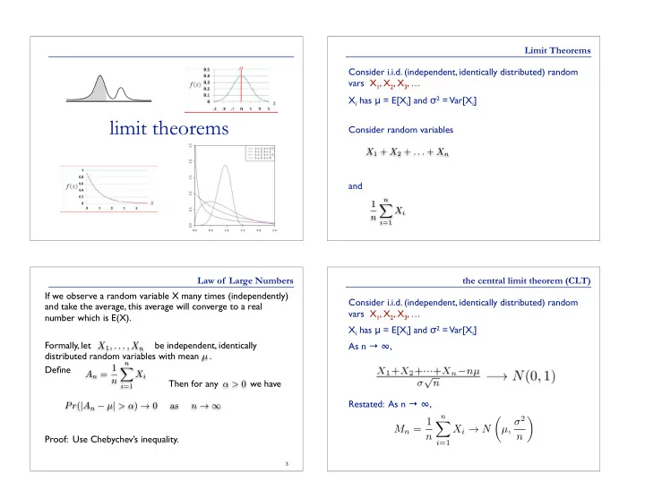
Limit Theorems Consider i.i.d. (independent, identically distributed) random vars X 1 , X 2 , X 3 , … X i has μ = E[X i ] and σ 2 = Var[X i ] limit theorems Consider random variables X 1 + X 2 + . . . + X n and n 1 X X i n i =1 Law of Large Numbers the central limit theorem (CLT) If we observe a random variable X many times (independently) Consider i.i.d. (independent, identically distributed) random and take the average, this average will converge to a real vars X 1 , X 2 , X 3 , … number which is E(X). X i has μ = E[X i ] and σ 2 = Var[X i ] Formally, let be independent, identically As n → ∞ , X 1 , . . . , X n distributed random variables with mean . µ n Define A n = 1 X X i n Then for any we have α > 0 i =1 Restated: As n → ∞ , Pr ( | A n − µ | > α ) → 0 as n → ∞ n µ, σ 2 ✓ ◆ M n = 1 X X i → N n n Proof: Use Chebychev’s inequality. i =1 3

CLT applies even to even wacky distributions 23 24 5 6 CLT in the real world CLT is the reason many things appear normally distributed Many quantities = sums of (roughly) independent random vars Exam scores: sums of individual problems People’s heights: sum of many genetic & environmental factors Measurements: sums of various small instrument errors ... 7 8

in the real world… in the real world… 9 10 in the real world… the central limit theorem (CLT) Consider i.i.d. (independent, identically distributed) random vars X 1 , X 2 , X 3 , … X i has μ = E[X i ] and σ 2 = Var[X i ] As n → ∞ , Restated: As n → ∞ , n µ, σ 2 ✓ ◆ M n = 1 X X i → N n n i =1 11

Example 1 Example 2 Number of students who enroll in a class is Poisson (100). If 10 fair die are rolled, find the approximate probability that Professor will teach course in two sections if more than 120 the sum obtained is between 30 and 40, inclusive, using CLT. students enroll. What is the probability of two sections? X i is the value of die # i. When applying approximation, use continuity correction: E(X i ) = 7/2 and Var(X i ) = 35/12 Think of Pr (X=i) = Pr (i-0.5 < X < i + 0.5) E ( X ) = 35 X = X 1 + X 2 + ...X 10 V ar ( X ) = 350 / 12 Recall Poisson (100) is sum of 100 independent Poisson(1) random variables, so we can apply CLT. ! 29 . 5 − 35 X − 35 ≤ 40 . 5 − 35 Pr (29 . 5 ≤ X ≤ 40 . 5) = Pr ≤ ✓ X − 100 ◆ p p p ≥ 119 . 5 − 100 350 / 12 350 / 12 350 / 12 Pr ( X > 119 . 5) = Pr √ √ 100 100 ≈ 2 · Φ (1 . 0184) − 1 ≈ 1 − Φ (1 . 95) ≈ 0 . 0256 . ≈ 0 . 692 . 13 14