
INF421, Lecture 7 Balanced Trees
Leo Liberti LIX, ´ Ecole Polytechnique, France
INF421, Lecture 7 – p. 1
Course
Objective: to teach you some data structures and associated
algorithms
Evaluation: TP noté en salle info le 16 septembre, Contrôle à la fin.
Note: max(CC, 3
4CC + 1 4TP)
Organization: fri 26/8, 2/9, 9/9, 16/9, 23/9, 30/9, 7/10, 14/10, 21/10,
amphi 1030-12 (Arago), TD 1330-1530, 1545-1745 (SI31,32,33,34)
Books:
- 1. Ph. Baptiste & L. Maranget, Programmation et Algorithmique, Ecole Polytechnique
(Polycopié), 2009
- 2. G. Dowek, Les principes des langages de programmation, Editions de l’X, 2008
- 3. D. Knuth, The Art of Computer Programming, Addison-Wesley, 1997
- 4. K. Mehlhorn & P
. Sanders, Algorithms and Data Structures, Springer, 2008 Website: www.enseignement.polytechnique.fr/informatique/INF421 Contact: liberti@lix.polytechnique.fr (e-mail subject: INF421)
INF421, Lecture 7 – p. 2
Lecture summary
Binary search trees AVL trees Heaps and priority queues Tries
INF421, Lecture 7 – p. 3
Notation
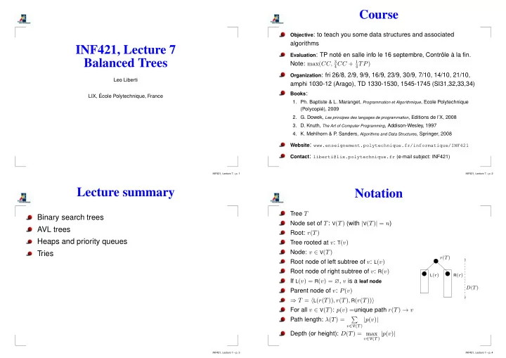
Tree T Node set of T: V(T) (with |V(T)| = n) Root: r(T) Tree rooted at v: T(v) Node: v ∈ V(T) Root node of left subtree of v: L(v) Root node of right subtree of v: R(v) If L(v) = R(v) = ∅, v is a leaf node Parent node of v: P(v) ⇒ T = L(r(T)), r(T), R(r(T)) For all v ∈ V(T): p(v) =unique path r(T) → v Path length: λ(T) =
- v∈V(T )
|p(v)| Depth (or height): D(T) = max
v∈V(T ) |p(v)|
r(T)
L(r) R(r)
D(T)
INF421, Lecture 7 – p. 4